Download as PDF, PPTX
![Terms - continued
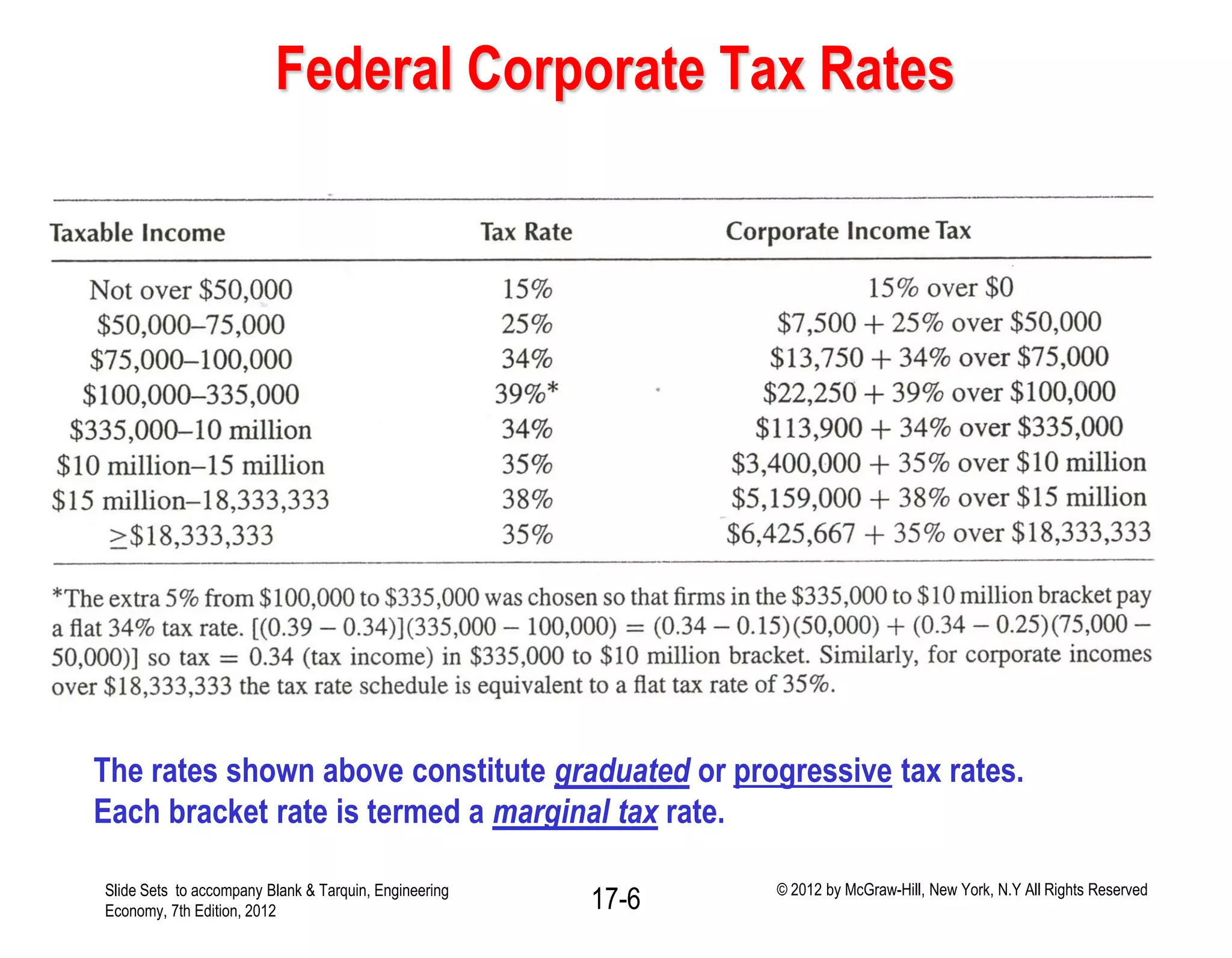
Tax rate T
A percentage or decimal
equivalent of TI.
For Federal corporate income
tax T is represented by a series
of tax rates.
The applicable tax rate depends
upon the total amount of TI.
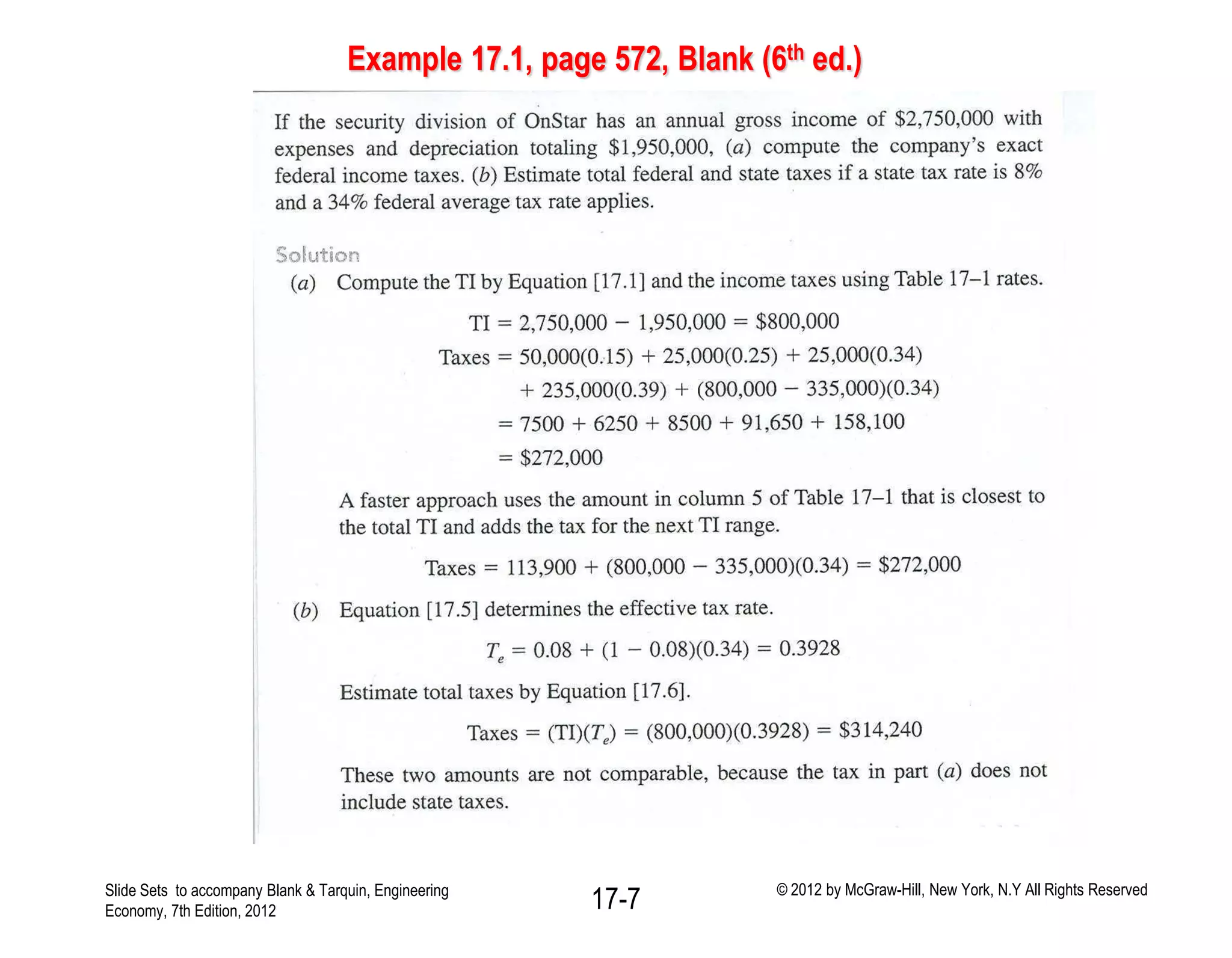
Taxes owed equals:
Taxes = (taxable income) x
(applicable rate)
= (TI)(T).
Net Profit After Tax (NPAT)
Amount of money remaining each year
when income taxes are subtracted from
taxable income.
NPAT = TI – {(TI)(T)}
= (TI)(1-T)
Effective tax rate Te combines federal and local
rates:
Total Tax = Federal tax + State tax
State tax is deductable from taxable federal
income, hence : if Tf is federal tax rate, Ts is
state tax rate, and Te is total effective tax rate:
TI (Te ) = TI(Ts) + [TI - TI(Ts)] (Tf)
Te = Tf + Ts – TfTs or Te = Ts + (1-Ts) Tf
Te = Tf + (1-Tf) Ts
Slide Sets to accompany Blank & Tarquin, Engineering
Economy, 7th Edition, 2012 17-4 © 2012 by McGraw-Hill, New York, N.Y All Rights Reserved](https://image.slidesharecdn.com/lecture9taxesandeva-140315184349-phpapp02/75/Lecture-9-taxes-and-eva-4-2048.jpg)
![Cash Flow After Tax (CFAT)
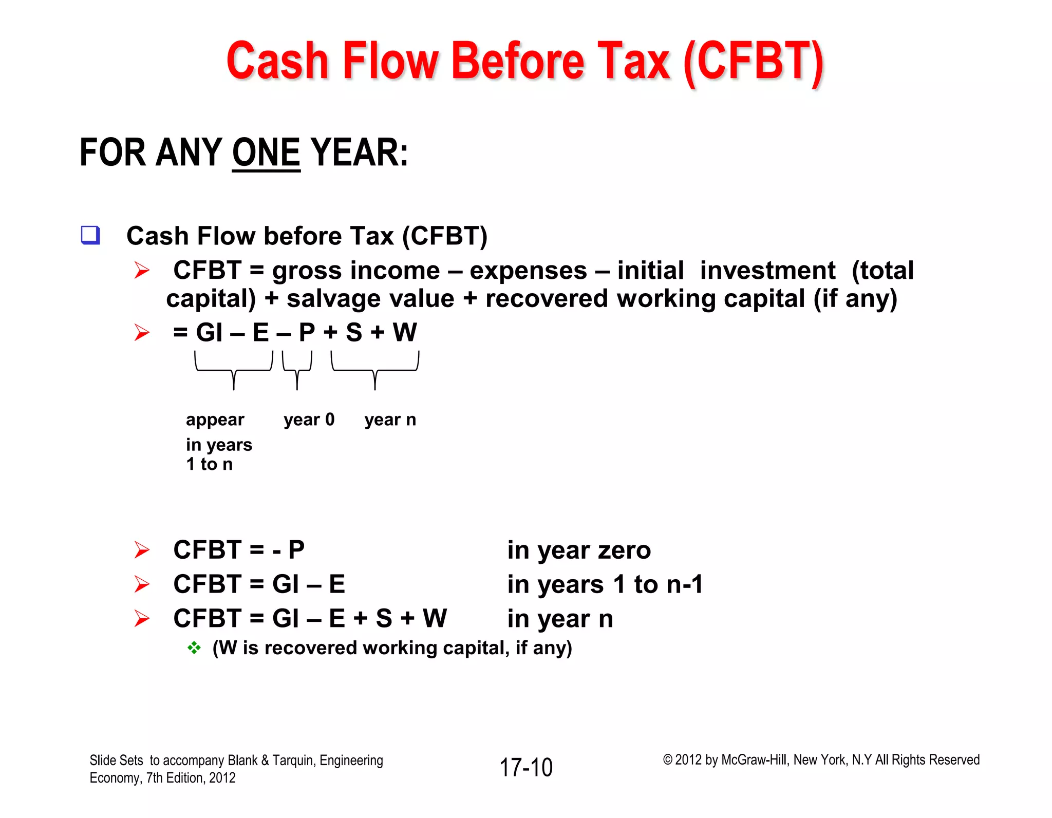
FOR ANY ONE YEAR:
Cash Flow After Tax (CFAT)
CFAT = CFBT – taxes
CFAT = [GI – E – P + S + W] – (GI – E – D)(Te)
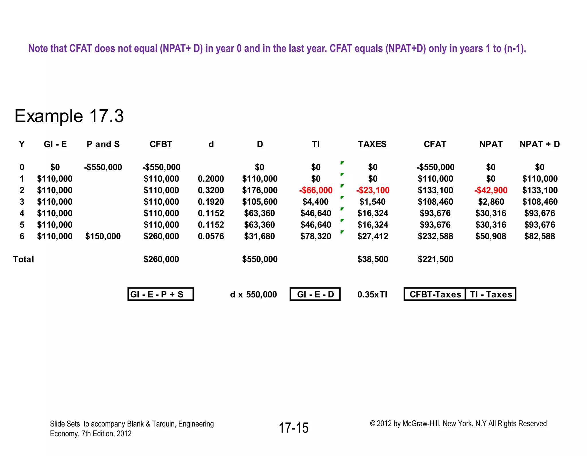
CFAT = NPAT + D Valid for all years except years 0 and n !
Note: only fixed capital is depreciable, if there is no working capital
then by definition total capital is fixed and is depreciable.
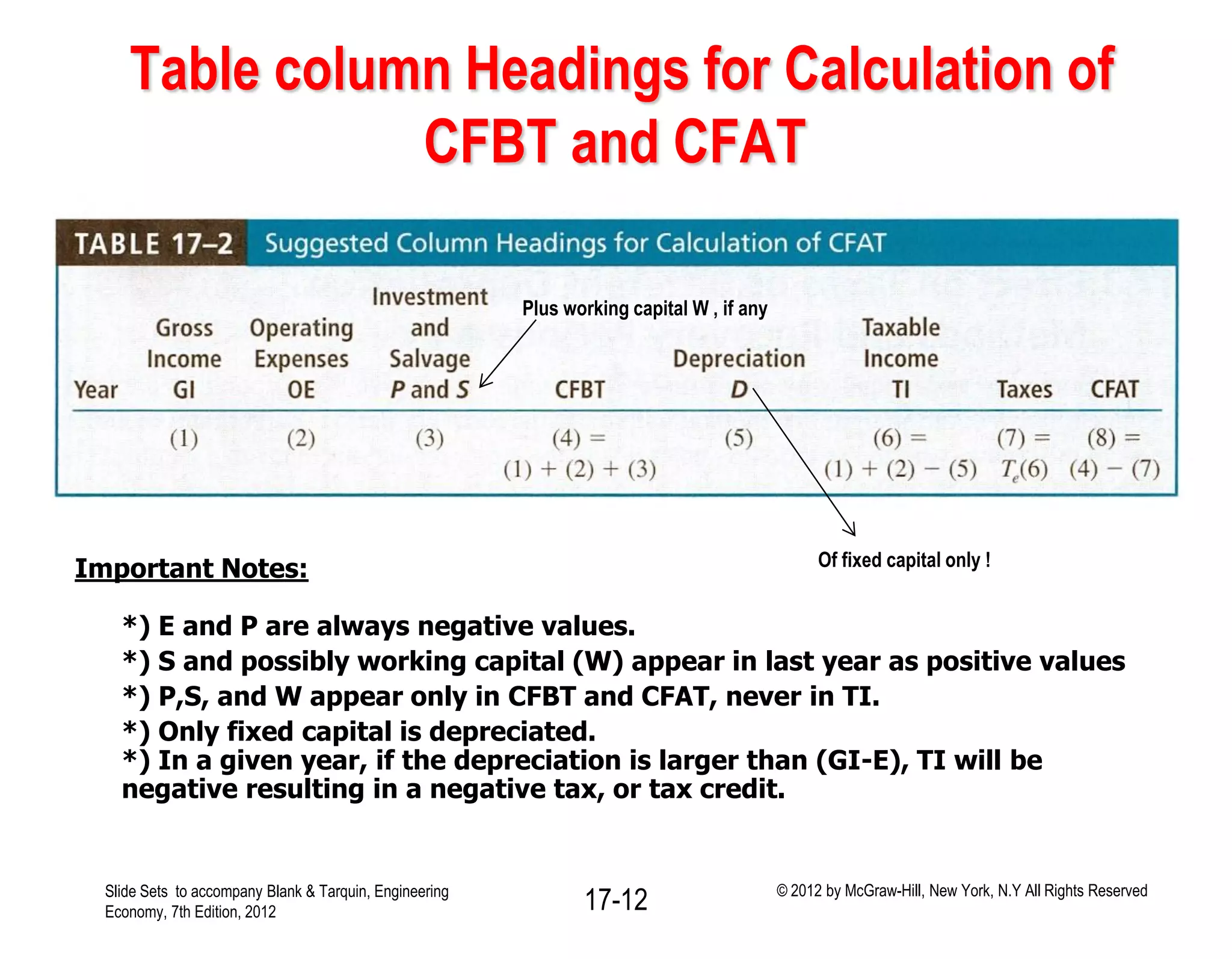
An evaluation format:
Table 17.2 , p. 449, Blank (7th ed.)
Slide Sets to accompany Blank & Tarquin, Engineering
Economy, 7th Edition, 2012 17-11 © 2012 by McGraw-Hill, New York, N.Y All Rights Reserved](https://image.slidesharecdn.com/lecture9taxesandeva-140315184349-phpapp02/75/Lecture-9-taxes-and-eva-11-2048.jpg)
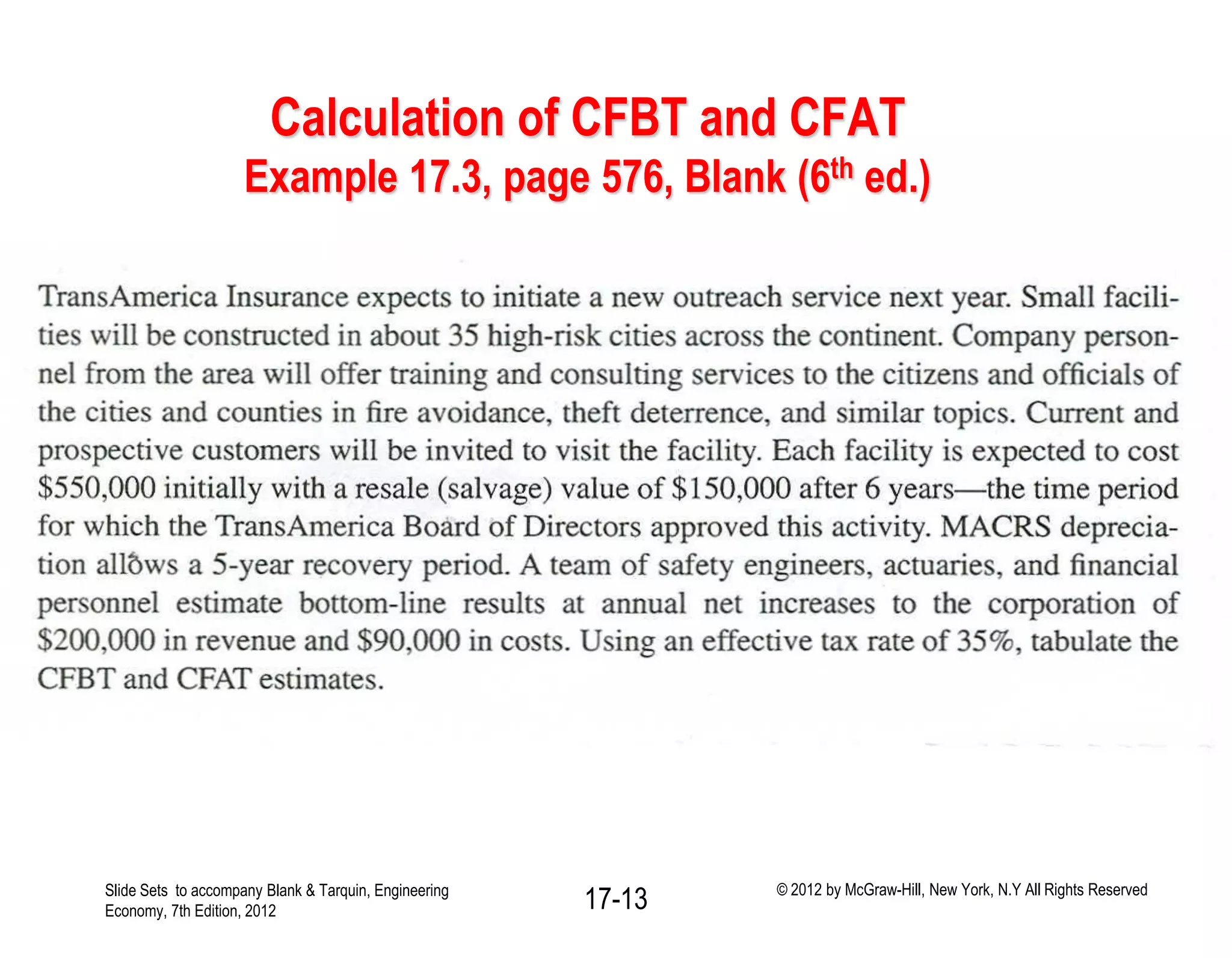
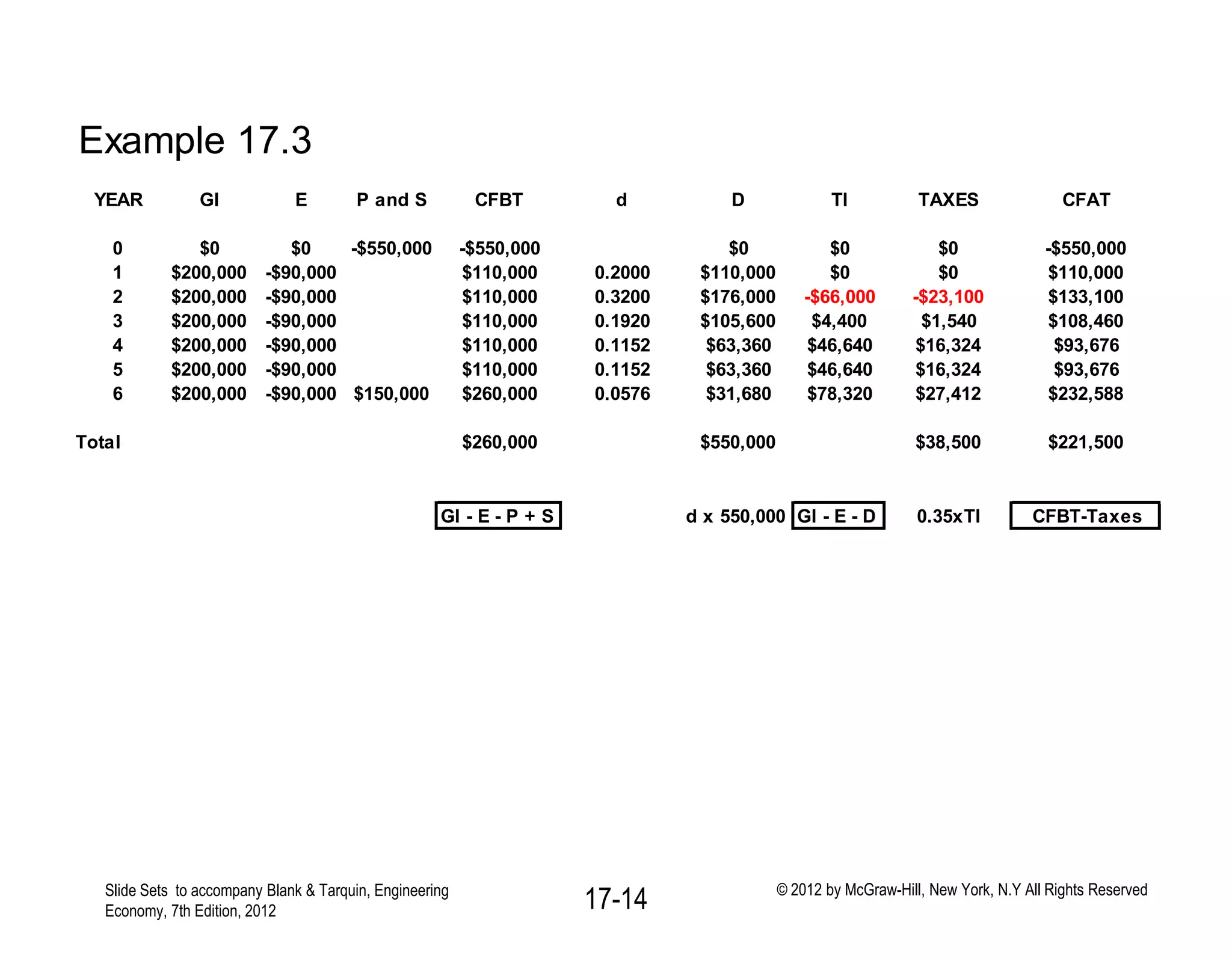
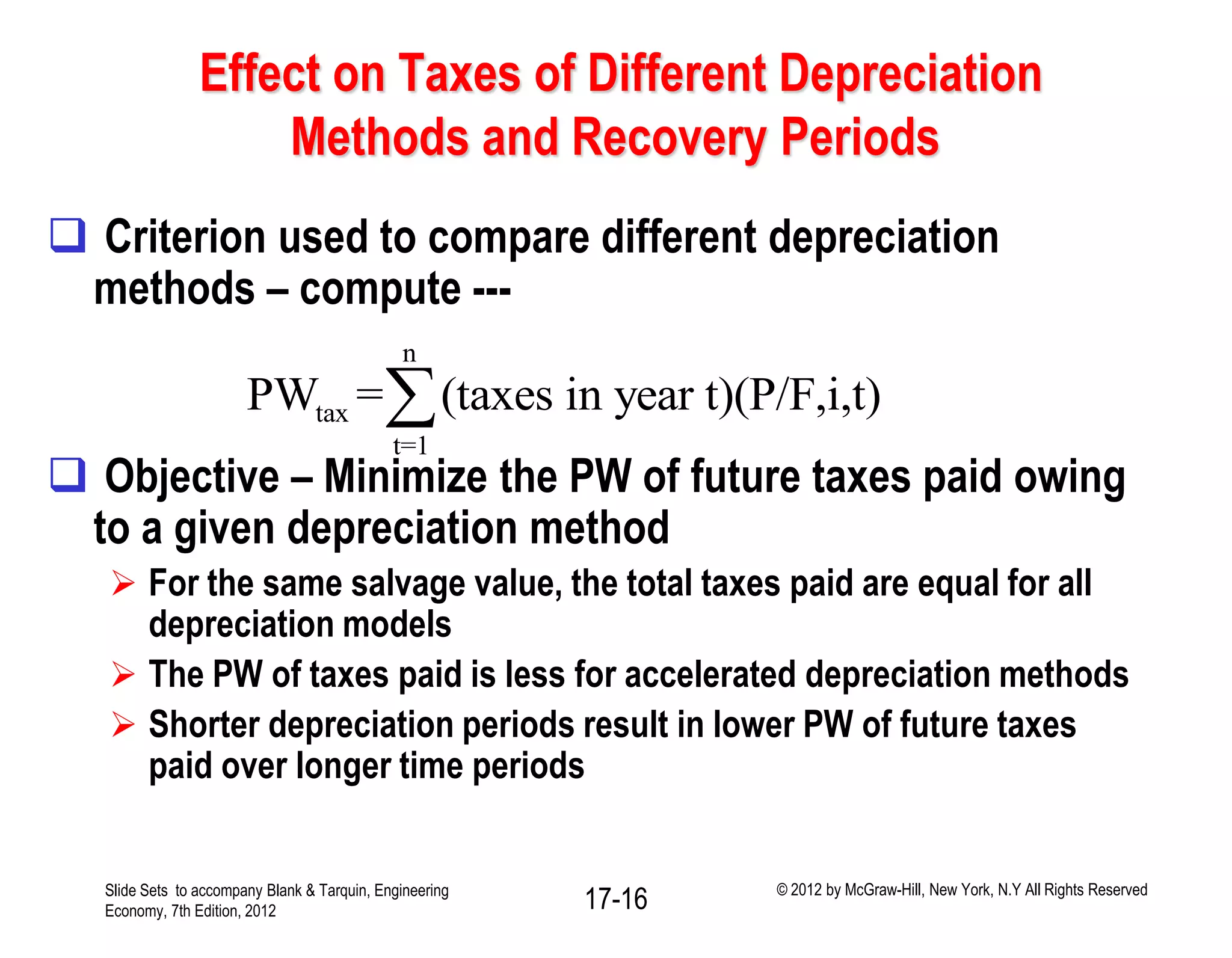
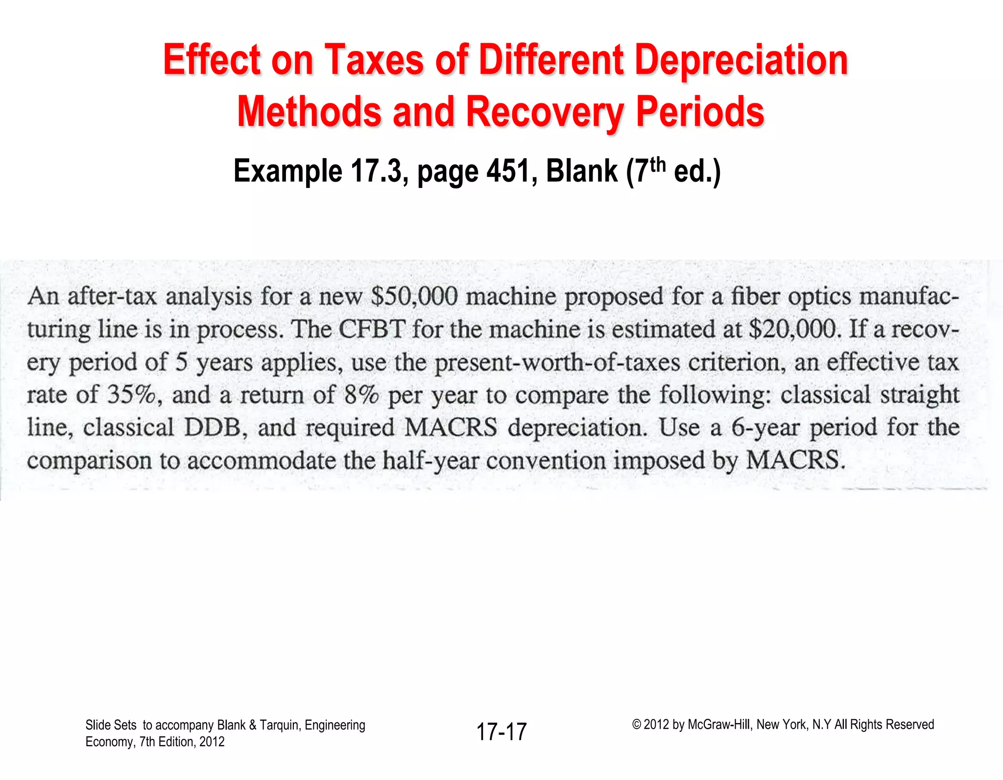
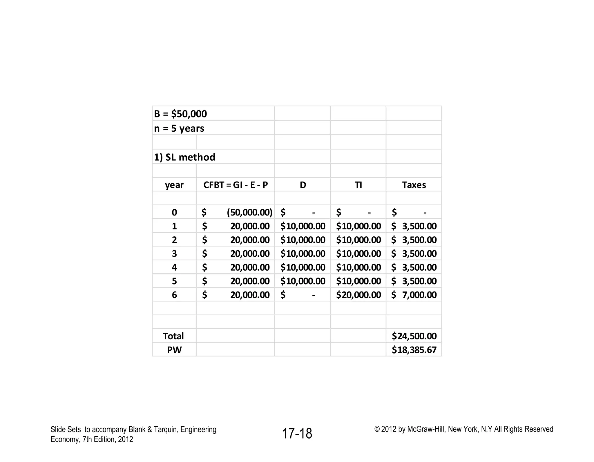
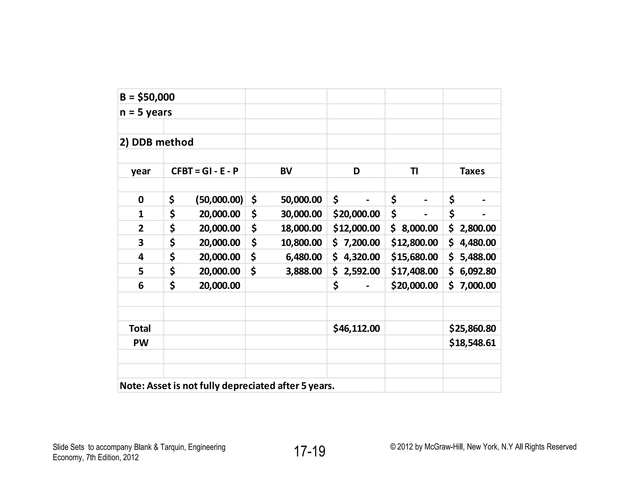
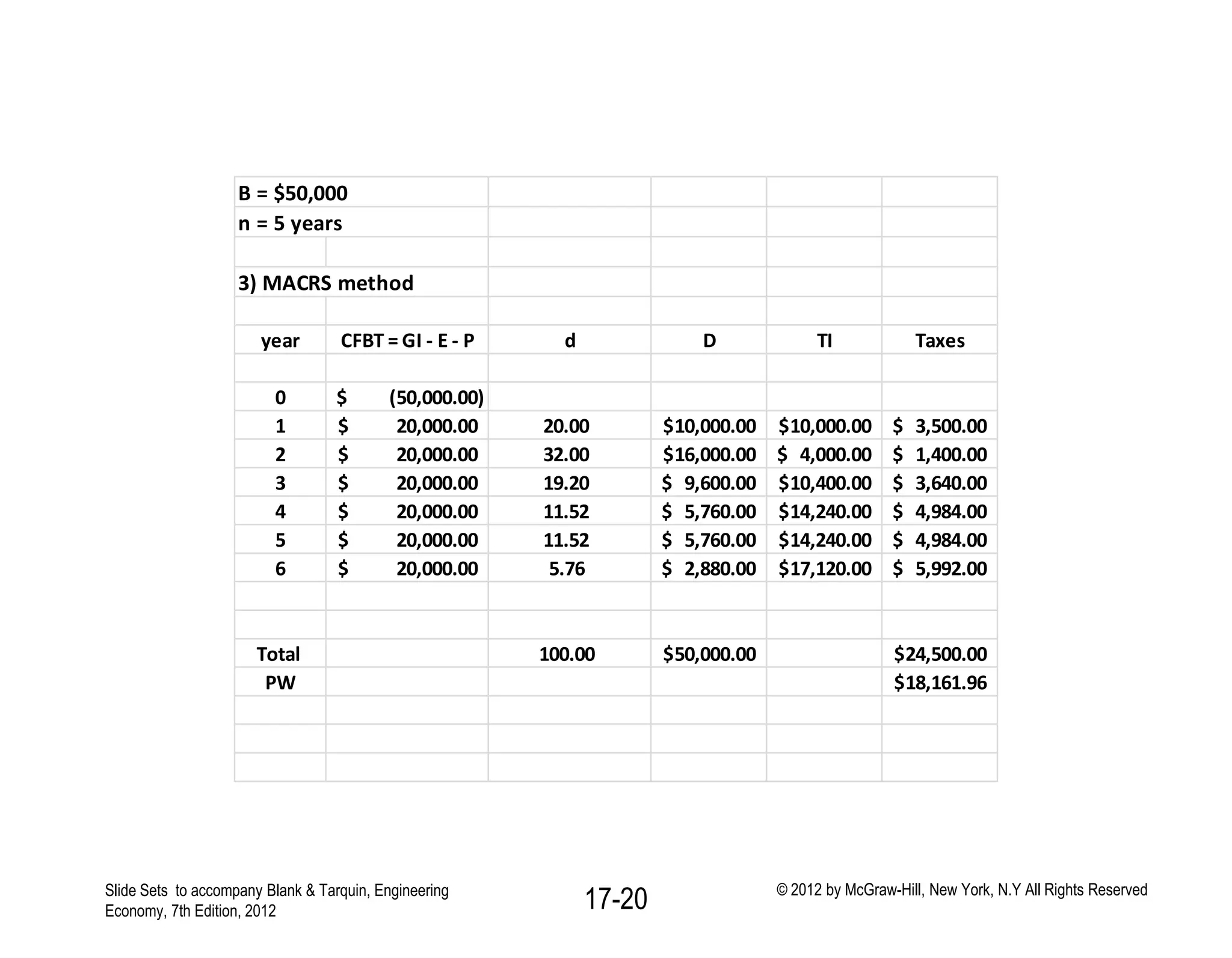
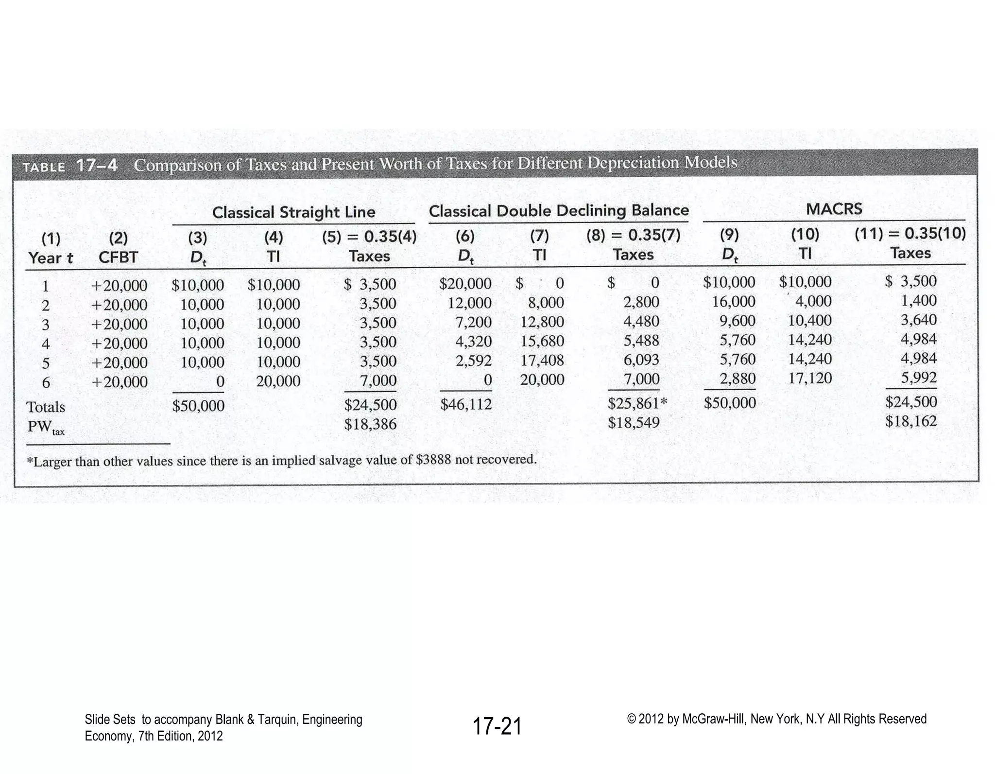
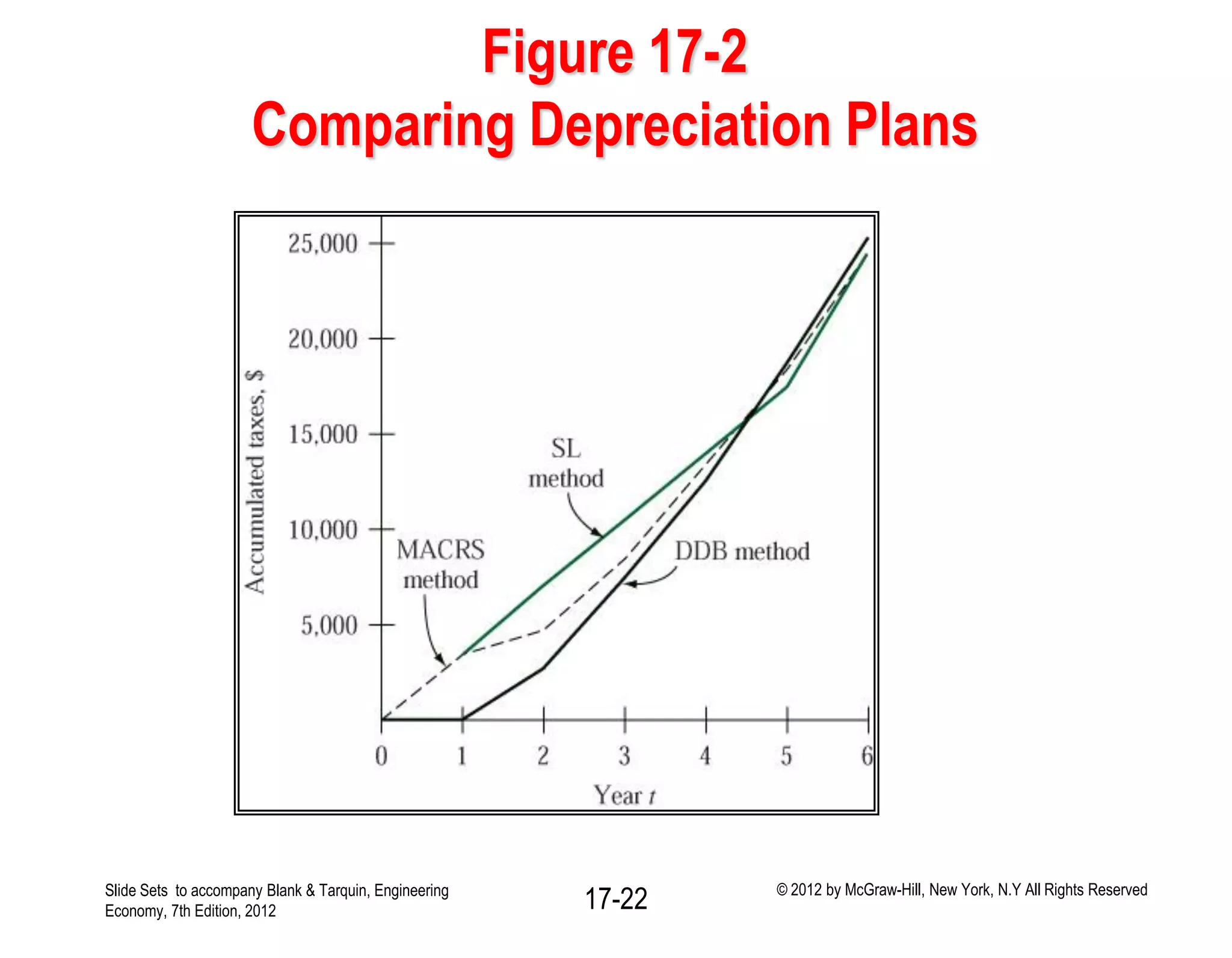
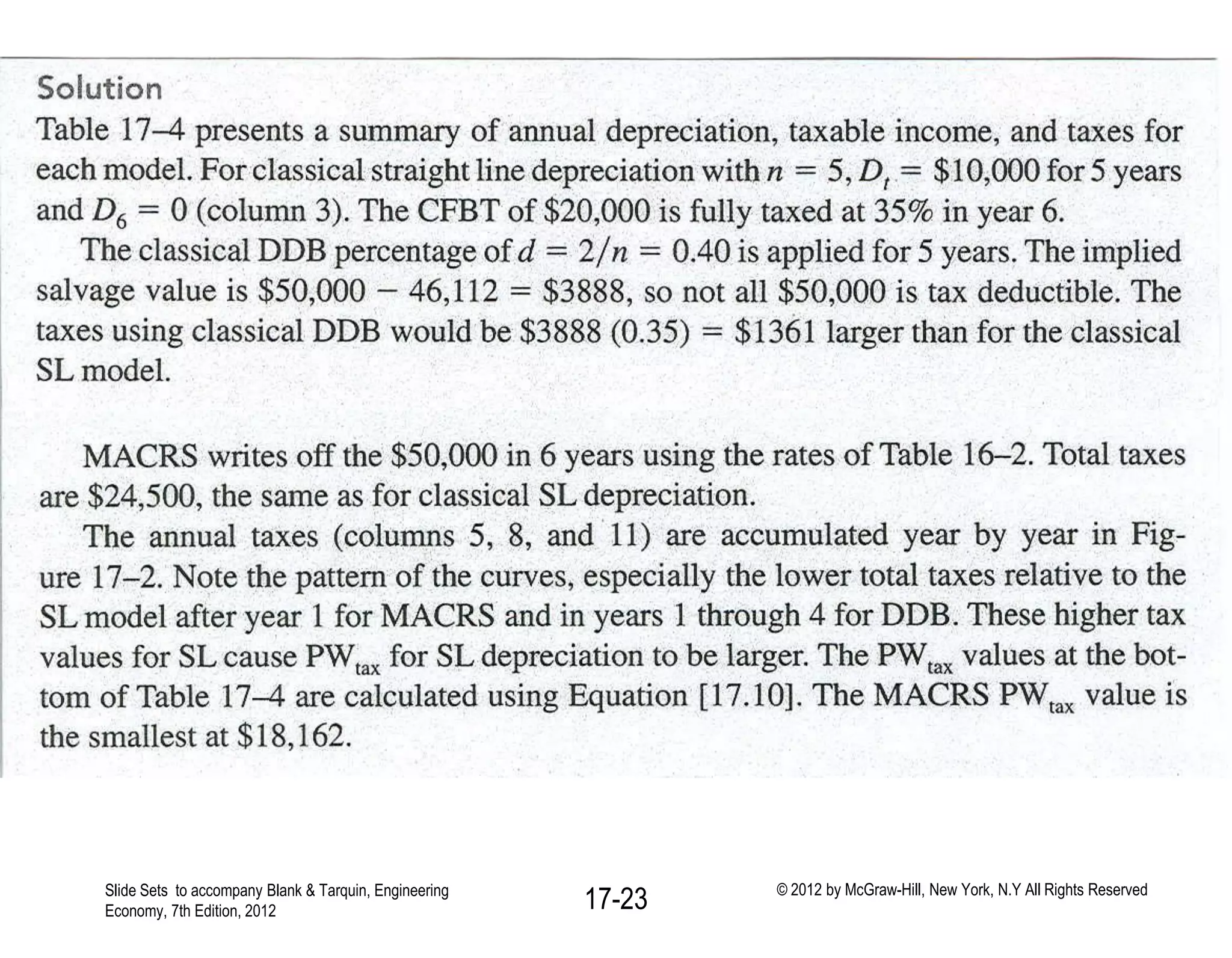

This document discusses concepts related to corporate income taxes and cash flow analysis. It defines key terms like gross income, taxable income, depreciation, taxes owed, and net profit after tax. It also discusses how to calculate cash flow before taxes and after taxes for each year of a project. The document provides an example cash flow analysis for a project using straight-line, double declining balance, and MACRS depreciation methods to demonstrate how different depreciation approaches can affect taxes paid over the life of a project. It emphasizes that accelerated depreciation methods and shorter recovery periods can lower the present value of total taxes paid.


