Download to read offline

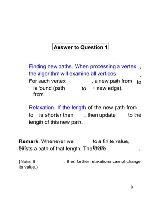
![Implementing the Idea of Relaxation
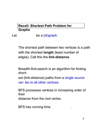
Consider an edge from a vertex to whose weight is
.
Suppose that we have already processed so that we know
and also computed a current estimate for
.
Then
There is a (shortest) path from
There is a path from
to
to
with length
with length
.
.
Combining this path from to with the edge
another path from to with length
, we obtain
.
If
, then we replace the old
with the new shorter path
. Hence we update
path
(originally,
s
).
w
d[v]
v
u
d[u]
10](https://image.slidesharecdn.com/148065320dijistraalgo-131205202150-phpapp01/85/148065320-dijistra-algo-10-320.jpg)
![The Selection in Dijkstra’s
Algorithm
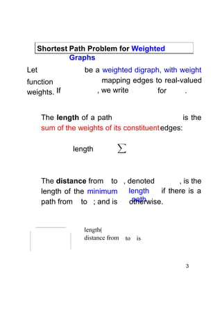
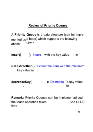
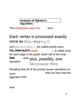
Question: How do we perform this selection
efficiently?
Answer: We store the vertices of
queue, where the key value of each
vertex
in a priority
is
.
[Note: if we implement the priority queue using a
heap,
we can perform the operations Insert(), time.]
Extract
and Decrease Key(), each in
Min(),
14](https://image.slidesharecdn.com/148065320dijistraalgo-131205202150-phpapp01/85/148065320-dijistra-algo-14-320.jpg)
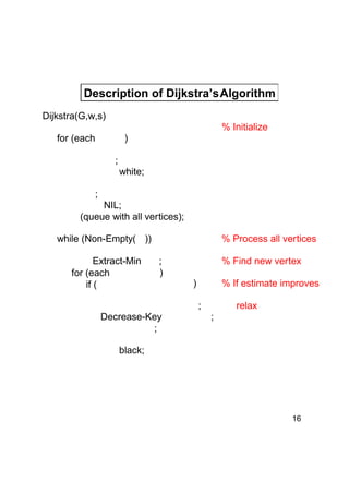
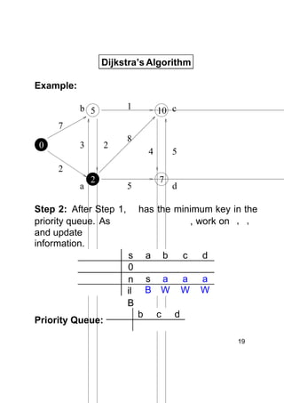
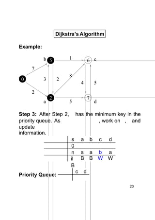
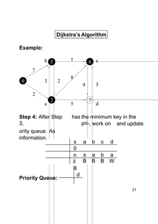
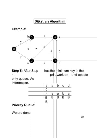
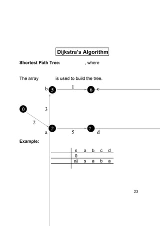

Dijkstra's algorithm finds the shortest paths from a single source vertex to all other vertices in a weighted graph. It uses a priority queue to iteratively select the vertex with the smallest estimated distance from the source. Each vertex is "relaxed" by examining its neighboring edges to find new shortest paths. When a vertex is removed from the queue, its distance estimate is guaranteed to be the true shortest path length. The algorithm runs in O(ElogV) time, where E is the number of edges and V is the number of vertices.


![Getting Started with Apache Spark: Big Data Made Simple [Free Meetup]](https://cdn.slidesharecdn.com/ss_thumbnails/apachesparkgettingstarted-260203175547-8361bcc3-thumbnail.jpg?width=640&height=640&fit=bounds)


