1D Elastoplasticity, Multi dimentional Elastoplasticity, Finite Rotation with Objective integration, Finite Deformation, Elasto-plasticity with Hyper elasticity, Mathematical Formulation, Finite Elasticity, Elasto-plasticity Analysis

1. 1
Prof. Samirsinh Parmar
Asst. Professor, Dept. of Civil Engg.
Dharmasinh Desai University, Nadiad, Gujarat, INDIA
Mail: samirddu@gmail.com
CHAPTER- 4

2. 2
Table of Contents
• 4.2. 1D Elastoplasticity
• 4.3. Multi-dimensional Elastoplasticity
• 4.4. Finite Rotation with Objective Integration
• 4.5. Finite Deformation Elastoplasticity with
Hyperelastcity
• 4.6. Mathematical Formulation from Finite Elasticity
• 4.7. MATLAB Code for Elastoplastic Material Model
• 4.8. Elastoplasticity Analysis Using Commercial Programs
• 4.9. Summary
• 4.10. Exercises

3. 3
1D Elastoplasticity
Section 4.2

4. 4
Goals
• Understand difference between elasticity and plasticity
• Learn basic elastoplastic model
• Learn different hardening models
• Understand different moduli used in 1D elastoplasticity
• Learn how to calculate plastic strain when total strain
increment is given
• Learn state determination for elastoplastic material

5. 5
Plasticity
• Elasticity – A material deforms under stress, but then
returns to its original shape when the stress is removed
• Plasticity - deformation of a material undergoing non-
reversible changes of shape in response to applied forces
– Plasticity in metals is usually a consequence of dislocations
– Rough nonlinearity
• Found in most metals, and in general is a good description
for a large class of materials
• Perfect plasticity – a property of materials to undergo
irreversible deformation without any increase in stresses
or loads
• Hardening - need increasingly higher stresses to result in
further plastic deformation

6. 6
Behavior of a Ductile Material
Terms Explanation
Proportional limit The greatest stress for which the stress is still proportional to
the strain
Elastic limit The greatest stress without resulting in any permanent strain on
release of stress
Young’s Modulus Slope of the linear portion of the stress-strain curve
Yield stress The stress required to produce 0.2% plastic strain
Strain hardening A region where more stress is required to deform the material
Ultimate stress The maximum stress the material can resist
Necking Cross section of the specimen reduces during deformation
Proportional
limit
Yield stress
Ultimate
stress
Strain
hardening
Necking
Fracture
s
e
Young’s
modulus

7. 7
Elastoplasticity
• Most metals have both elastic and plastic properties
– Initially, the material shows elastic behavior
– After yielding, the material becomes plastic
– By removing loading, the material becomes elastic
• We will assume small (infinitesimal) deformation case
– Elastic and plastic strain can be additively decomposed by
– Strain energy density exists in terms of elastic strain
– Stress is related to the elastic strain, not the plastic strain
• The plastic strain will be considered as an internal
variable, which evolves according to plastic deformation
e p
e  e  e
2
1
0 e
2
U E( )
 e

8. 8
1D Elastoplasticity
• Idealized elastoplastic stress-strain behavior
– Initial elastic behavior with slope E (elastic modulus) until yield
stress σY (line o–a)
– After yielding, the plastic phase with slope Et (tangent modulus)
(line a–b).
– Upon removing load, elastic unloading
with slope E (line b-c)
– Loading in the opposite direction,
the material will eventually yield
in that direction (point c)
– Work hardening – more force is
required to continuously deform
in the plastic region (line a-b or c-d)
a
b
d
e
σ
ε
c
o
E
Et

9. 9
Work Hardening Models
• Kinematic hardening
– Elastic range remains constant
– Center of the elastic region moves
parallel to the work hardening line
– bc = de = 2oa
– Use the center of elastic domain
as an evolution variable
• Isotropic hardening
– Elastic range (yield stress) increases
proportional to plastic strain
– The yield stress for the reversed loading
is equal to the previous yield stress
– Use plastic strain as an evolution
variable
• No difference in proportional loading (line o-a-b)
a
b
d
e
σ
ε
c
o
a
b
d
e
σ
ε
c
o
h
h

10. 10
Elastoplastic Analysis
• Additive decomposition
– Only elastic strain contributes to stress (but we don’t know how
much of the total strain corresponds to the elastic strain)
– Let’s consider an increment of strain:
– Elastic strain increases stress by
– Elastic strain disappears upon removing loads or changing direction
Elastic
slope, E
σ
ε
E
σY
εY
Strain hardening slope, Et
Δσ
Δε
Δεp
Δεe
Reloading
σ
ε
E
Initial loading
E
Unloading
e p
e  e  e
e
E
s  e

11. 11
Elastoplastic Analysis cont.
• Additive decomposition (continue)
– Plastic strain remains constant during unloading
– The effect of load-history is stored in the plastic strain
– The yield stress is determined by the magnitude of plastic strain
– Decomposing elastic and plastic part of strain is an important
part of elastoplastic analysis
• For given stress s, strain cannot be determined.
– Complete history is required (path- or history-dependent)
– History is stored in evolution variable (plastic strain)
σ
ε
o

12. 12
Plastic Modulus
• Strain increment
• Stress increment
• Plastic modulus
• Relation between moduli
• Both kinematic and isotropic hardenings have the same
plastic modulus
e
E
s  e
p
H
s

e
e p t
E H E
s  e  e  e
t t
1 1 1
E E H E E H
s s s
    
t
t
EE
H
E E

 t
EH E
E E 1
E H E H
 
  
 
 
 
σ
ε
E
σY
εY
Strain hardening slope, Et
Δσ
Δε
Δεp
Δεe
e p
e  e  e
Et
H
ep
ee

13. 13
Analysis Procedure
• Analysis is performed with a given incremental strain
– N-R iteration will provide u e
– But, we don’t know ee or ep
• When the material is in the initial elastic range, regular
elastic analysis procedure can be used
• When the material is in the plastic range, we have to
determine incremental plastic strain
p
e p p p
p
p
H
E E
H
1
E
1 H / E
e
s
e  e  e   e   e
 
 e 
 
 
e
 e 

σ
ε
E
σY
εY
Δσ
Δε
Δεp
Δεe
Only when the material is on the plastic curve!!

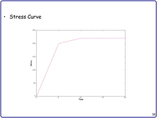
14. 14
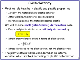
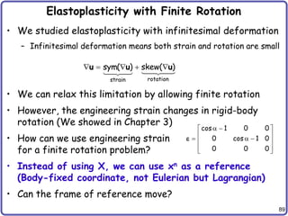
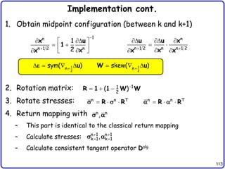
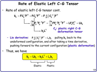
1D Finite Element Formulation
• Load increment
– applied load is divided by N increments: [t1, t2, …, tN]
– analysis procedure has been completed up to load increment tn
– a new solution at tn+1 is sought using the Newton-Raphson method
– iteration k has been finished and the current iteration is k+1
• Displacement increments
– From last increment tn:
– From previous iteration:
x1 x2
u1 u2
P1 P2
L
k n 1 k n
k n 1 k 1 n 1 k

  
  
  
d d d
d d d
1
2
u
u
 
  
 
d

15. 15
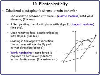
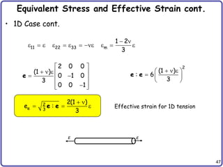
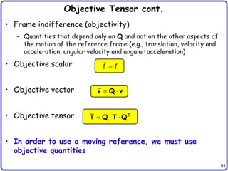
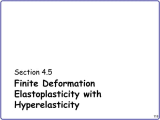
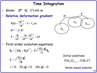
1D FE Formulation cont.
• Interpolation
• Weak form (1 element)
– Internal force = external force
1
1 2
2
u
u(x) [N N ]
u

 
    
 

 
N d
  1
2
u
d 1 1
u
dx L L u

 
 
e       
 
  
   
B d
u
   
e   
N d
B d
L
T T n 1 k 1 T n 1 2
0
Adx , R
  
s   

d B d F d 1
2
u
u
 
  
 
d

16. 16
1D FE Formulation cont.
• Stress-strain relationship (Incremental)
– Elastoplastic tangent modulus
• Linearization of weak form
ep
n 1 k 1 n 1 k n 1 k
D
   
s
s  s  e  s  e
e
ep
t
E if elastic
D
E if plastic

 

L L
ep
T T T T T n 1 k
0 0
D Adx Adx

     s
 
 
 
d B B d d F d B
Tangent stiffness Residual

17. 17
1D FE Formulation cont.
• Tangent Stiffness
• Residual
• State Determination:
• Incremental Finite Element Equation
– N-R iteration until the residual vanishes
ep
T
1 1
AD
L 1 1

 
  

 
k
n 1 n 1 k
L 1
n 1 k n 1 T n 1 k
n 1 n 1 k
0
2
F A
Adx
F A
 
  
 
 
 s
 
  s   
 s
 
 

R F B
n 1 k n n k
p
f( , , , )

s  s e e
k n 1 k
T

  
k d R

18. 18
Isotropic Hardening Model
• Yield strength gradually increases proportional to the
plastic strain
– Yield strength is always positive for both tension or compression
– Plastic strain is always positive and continuously accumulated even
in cycling loadings
n 0 n
Y Y p
H
s  s  e Initial yield stress
Total plastic strain
σ
ε
E
n
Y
s
0
Y
s
εe
εp
ε
E
n
Y
s
0
Y
s
εp
n
Y
s
1

n
Y
s
σ

19. 19
State Determination (Isotropic Hardening)
• How to determine stress
– Given: strain increment (Δe) and all variables in load step n
1. Computer current yield stress
2. Elastic predictor
3. Check yield status
n 0 n
Y Y p
H
s  s  e
tr
E
s  e tr n tr
s  s  s
tr tr n
y
f  s  s
Trial yield function
σ
ε
E
a b
c
d e
f
σn+1
n
Y
s
0
Y
s
σn
σtr
Δσtr
Δε
Δεep= (1–R)Δε
Δεp
RΔσtr
tr
f (1 R)E
  e
0 n n
Y p
(E,H, , , )
s s e

20. 20
State Determination (Isotropic Hardening) cont.
• If , material is elastic
• If , material is plastic (yielding)
Either transition from elastic to plastic or continuous yielding
– Stress update (return to the yield surface)
– Update plastic strain
tr
f 0

n 1 tr

s  s
σ
ε
E
Initial loading
Unloading
Reloading
Either initial elastic region or unloading
tr
f 0

n 1 tr tr
p
sgn( )E

s  s  s e
n 1 n
p p p

e  e  e
Plastic strain increment is unknown
e p
e  e  e
For a given strain increment, how much is elastic and plastic?

21. 21
State Determination (Isotropic Hardening) cont.
• Plastic consistency condition
– to determine plastic strain increment
– Stress must be on the yield surface after plastic deformation
n 1 n 1 n 1
y
f 0
  
 s  s 
tr tr n
p y p
tr n
y p
sgn( )E ( H ) 0
(E H) 0
 s  s e  s  e 
 s  s   e 
tr n tr
y
p
f
E H E H
s  s
e  
 
p
E
(1 R)
E H
e   e

σ
ε
E
a b
c
d e
f
σn+1
n
Y
s
0
Y
s
σn
σtr
Δσ
Δε
Δεep= (1–R)Δε
Δεp
RΔσ
%Note: ep is always positive!!
tr
tr
f
R 1
 
s

22. 22
State Determination (Isotropic Hardening) cont.
• Update stress
• Algorithm
1) Elastic trial
2) Plastic return mapping
– No iteration is required in linear hardening models
Elastic trial Plastic compensation
(return mapping)
n 1 tr tr
p
2
n 1 tr tr
sgn( )E
(1 R)E
sgn( )
E H


s  s  s e

s  s  s e

σ
ε
E
a b
c
d e
f
σn+1
n
Y
s
0
Y
s
σn
σtr
Δσ
Δε
Δεep= (1–R)Δε
Δεp
RΔσ

23. 23
Algorithmic Tangent Stiffness
• Continuum tangent modulus
– The slope of stress-strain curve
• Algorithmic tangent modulus
– Differentiation of the state determination algorithm
• Dalg = Dep for 1D plasticity!!
– We will show that they are different for multi-dimension
ep
t
E if elastic
D
E if plastic

 

tr
p
alg tr
D sgn( )E
e
s  s
   s
e e e
tr
p tr
1 f E
sgn( )
E H E H
e 
  s
e  e 
alg
t
E if elastic
D
E if plastic

 


24. 24
Algorithm for Isotropic Hardening
• Given:
1. Trial state
1. If (elastic)
– Remain elastic: ; exit
2. If (plastic)
a. Calculate plastic strain:
b. Update stress and plastic strain (store them for next increment)
tr n
n 0 n
Y Y p
tr tr n
Y
E
H
f
s  s  e
s  s  e
 s  s
0 n n
Y p
, E, H, , ,
e s s e
n 1 tr n 1 n
p p
,
 
s  s e  e
tr
f 0

tr
f 0

tr
p
f
E H
e 

n 1 tr tr
p
sgn( )E

s  s  s e n 1 n
p p p

e  e  e

25. 25
Ex) Elastoplastic bar
• E = 200GPa, H = 25GPa, 0sy = 250MPa
• ns = 150MPa, nep = 0.0001, e = 0.002
• Yield stress:
– Material is elastic at tn
• Trial stress:
• Plastic consistency condition
• State update
n 0 n
Y Y p
H 252.5MPa
s  s  e 
tr
tr n tr
E 400MPa
550MPa
 s  e 
s  s   s  Now material is plastic
tr
3
p
f
1.322 10
E H

e   

n 1 tr tr
p
sgn( )E 285.6MPa

s  s  s e 
n 1 n 3
p p p 1.422 10
 
e  e  e  

26. 26
Kinematic Hardening Model
• Yield strength remains constant, but the center of elastic
region moves parallel to the hardening curve
• Effective stress is defined using the shifted stress
• Use the center of elastic domain as an evolution variable
n 1 n
p
sgn( )H

     e Back stress
  s  
σ
ε
E
n
s
0
Y
s
εe
εp
n

0
Y
s
σ
ε
E
n
s
0
Y
s
2εp
1

n

0
2 Y
s

27. 27
State Determination (Kinematic Hardening)
• Given: Material properties and state at increment n:
• Elastic predictor
• Check yield status
• If , material is elastic
• If , material is plastic (yielding)
0 n n n
Y p
( ,E,H, , , , )
e s s  e
tr n tr n tr tr tr
E , ,
s  s  e      s  
tr tr 0
y
f    s
Trial yield function
tr
f 0

n 1 tr

s  s
Either initial elastic region or unloading
tr
f 0

Either transition from elastic to plastic or continuous yielding
σ
ε
E
a b
c
d e
σn+1
σn
σtr
Δε
αn
tr
αn+1
f
g

28. 28
State Determination (Kinematic Hardening) cont.
• Updating formulas for stress, back stress & plastic strain
• Plastic consistency condition
– To determine unknown plastic strain increment
– Stress must be on the yield surface during plastic loading
n 1 tr tr
p
sgn( )E

s  s   e n 1 n
p p p

e  e  e
n 1 tr tr
p
sgn( )H

     e
n 1 n 1 0
y
f 0
 
   s 
tr tr tr tr 0
p p y
tr tr 0
y p
sgn( )E sgn( )H 0
(E H) 0
 s   e     e  s 
 s    s   e 
tr n tr
y
p
f
E H E H
  s
e  
 
%Note: the same formula with
isotropic hardening model!!

29. 29
Algorithm for Kinematic Hardening
• Given:
1. Trial state
2. If (elastic)
– Remain elastic: ; exit
3. If (plastic)
a. Calculate plastic strain:
b. Update stress and plastic strain (store them for next increment)
tr n
tr n
tr tr tr
tr tr 0
Y
E
f
s  s  e
  
  s  
   s
n 1 tr n 1 n n 1 n
p p
, ,
  
s  s    e  e
tr
f 0

tr
f 0

tr
p
f
E H
e 

n 1 tr tr
p
sgn( )E

s  s   e
n 1 n
p p p

e  e  e
0 n n n
Y p
,E,H, , , ,
e s s  e
n 1 n tr
p
sgn( )H

     e

30. 30
Combined Hardening Model
• Baushinger effect
– conditions where the yield strength of a metal decreases when the
direction of strain is changed
– Common for most polycrystalline metals
– Related to the dislocation structure in the cold worked metal. As
deformation occurs, the dislocations will accumulate at barriers
and produce dislocation pile-ups and tangles.
• Numerical modeling of Baushinger effect
– Modeled as a combined kinematic and isotropic hardening
n 1 n
Y Y p
(1 )H

s  s    e n 1 n
p
sgn( ) H

      e
 = 0: isotropic hardening
 = 1: kinematic hardening
0 1
  

31. 31
Combined Hardening Model cont.
• Trial state
• Stress update
• Show that the plastic increment is the same
tr n
tr n
tr tr tr
tr tr 0
Y
E
f
s  s  e
  
  s  
   s
n 1 tr tr
p
n 1 tr tr
p
n 1 n
Y y p
sgn( )E
sgn
1
( ) H
H
( )



s  s  

e


    e
s  
s  e
tr
p
f
E H
e 


32. 32
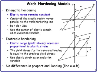
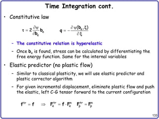
MATLAB Program combHard1D
%
% 1D Linear combined isotropic/kinamtic hardening model
%
function [stress, alpha, ep]=combHard1D(mp, deps, stressN, alphaN, epN)
% Inputs:
% mp = [E, beta, H, Y0];
% deps = strain increment
% stressN = stress at load step N
% alphaN = back stress at load step N
% epN = plastic strain at load step N
%
E=mp(1); beta=mp(2); H=mp(3); Y0=mp(4); %material properties
ftol = Y0*1E-6; %tolerance for yield
stresstr = stressN + E*deps; %trial stress
etatr = stresstr - alphaN; %trial shifted stress
fyld = abs(etatr) - (Y0+(1-beta)*H*epN); %trial yield function
if fyld < ftol %yield test
stress = stresstr; alpha = alphaN; ep = epN;%trial states are final
return;
else
dep = fyld/(E+H); %plastic strain increment
end
stress = stresstr - sign(etatr)*E*dep; %updated stress
alpha = alphaN + sign(etatr)*beta*H*dep; %updated back stress
ep = epN + dep; %updated plastic strain
return;

33. 33
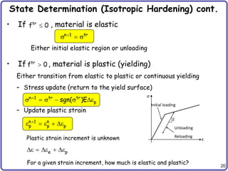
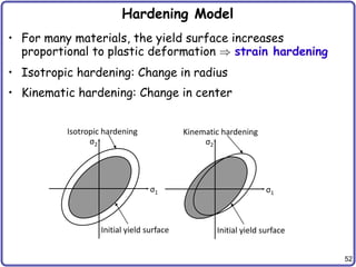
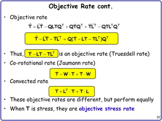
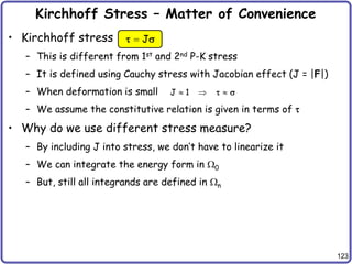
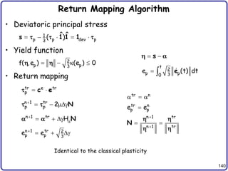
Ex) Two bars in parallel
• Bar 1: A = 0.75, E = 10000, Et = 1000, 0sY = 5, kinematic
• Bar 2: A = 1.25, E = 5000, Et = 500, 0sY = 7.5, isotropic
• MATLAB program
%
% Example 4.5 Two elastoplastic bars in parallel
%
E1=10000; Et1=1000; sYield1=5;
E2=5000; Et2=500; sYield2=7.5;
mp1 = [E1, 1, E1*Et1/(E1-Et1), sYield1];
mp2 = [E2, 0, E2*Et2/(E2-Et2), sYield2];
nS1 = 0; nA1 = 0; nep1 = 0;
nS2 = 0; nA2 = 0; nep2 = 0;
A1 = 0.75; L1 = 100;
A2 = 1.25; L2 = 100;
tol = 1.0E-5; u = 0; P = 15; iter = 0;
Res = P - nS1*A1 - nS2*A2;
Dep1 = E1; Dep2 = E2;
conv = Res^2/(1+P^2);
fprintf('niter u S1 S2 A1 A2');
fprintf(' ep1 ep2 Residual');
fprintf('n %3d %7.4f %7.3f %7.3f %7.3f %7.3f %8.6f %8.6f %10.3e',...
iter,u,nS1,nS2,nA1,nA2,nep1,nep2,Res);
Bar1
Bar2
Rigid 15

34. 34
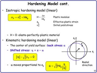
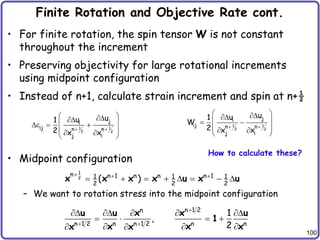
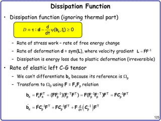
Ex) Two bars in parallel cont.
while conv > tol && iter < 20
delu = Res / (Dep1*A1/L1 + Dep2*A2/L2);
u = u + delu;
delE = delu / L1;
[Snew1, Anew1, epnew1]=combHard1D(mp1,delE,nS1,nA1,nep1);
[Snew2, Anew2, epnew2]=combHard1D(mp2,delE,nS2,nA2,nep2);
Res = P - Snew1*A1 - Snew2*A2;
conv = Res^2/(1+P^2);
iter = iter + 1;
Dep1 = E1; if epnew1 > nep1; Dep1 = Et1; end
Dep2 = E2; if epnew2 > nep2; Dep2 = Et2; end
nS1 = Snew1; nA1 = Anew1; nep1 = epnew1;
nS2 = Snew2; nA2 = Anew2; nep2 = epnew2;
fprintf('n %3d %7.4f %7.3f %7.3f %7.3f %7.3f %8.6f %8.6f %10.3e',...
iter,u,nS1,nS2,nA1,nA2,nep1,nep2,Res);
end
Iteration u s1 s2 ep1 ep2 Residual
0 0.0000 0.000 0.000 0.000000 0.000000 1.50E+1
1 0.1091 5.591 5.455 0.000532 0.000000 3.99E+0
2 0.1661 6.161 7.580 0.001045 0.000145 9.04E 1
3 0.2318 6.818 7.909 0.001636 0.000736 0.00E+0

35. 35
Summary
• Plastic deformation depends on load-history and its
information is stored in plastic strain
• Stress only depends on elastic strain
• Isotropic hardening increases the elastic domain, while
kinematic hardening maintain the size of elastic domain
but moves the center of it
• Major issue in elastoplastic analysis is to decompose the
strain into elastic and plastic parts
• Algorithmic tangent stiffness is consistent with the state
determination algorithm
• State determination is composed of (a) elastic trial and (b)
plastic return mapping

36. 36
1D Elastoplastic Analysis Using ABAQUS
• Material Card
*MATERIAL,NAME=ALLE
*ELASTIC
200.E3,.3
*PLASTIC
200.,0.
220.,.0009
220.,.0029
Yield stress
Plastic strain

37. 37
1D Elastoplastic Analysis Using ABAQUS
*HEADING
UniaxialPlasticity
*NODE,NSET=ALLN
1,0.,0.,0.
2,1.,0.,0.
3,1.,1.,0.
4,0.,1.,0.
5,0.,0.,1.
6,1.,0.,1.
7,1.,1.,1.
8,0.,1.,1.
*ELEMENT,TYPE=C3D8,ELSET=ALLE
1,1,2,3,4,5,6,7,8
*SOLID SECTION,ELSET=ALLE,MATERIAL=ALLE
*MATERIAL,NAME=ALLE
*ELASTIC
200.E3,.3
*PLASTIC
200.,0.
220.,.0009
220.,.0029
*BOUNDARY
1,PINNED
2,2
5,2
6,2
4,1
5,1
8,1
2,3
3,3
4,3
*STEP,INC=20
*STATIC,DIRECT
1.,20.
*BOUNDARY
7,3,,.004
5,3,,.004
6,3,,.004
8,3,,.004
*EL PRINT,FREQ=1
S,
E,
EP,
*NODE PRINT
U,RF
*END STEP

38. 38
• Stress Curve

39. 39
Multi-Dimensional
Elastoplastic Analysis
Section 4.3

40. 40
Goals
• Understand failure criteria, equivalent stress, and
effective strain
• Understand how 1D tension test data can be used for
determining failure of 3D stress state
• Understand deviatoric stress and strain
• Understand the concept of elastic domain and yield
surface
• Understand hardening models
• Understand evolution of plastic variables along with that
of the yield surface

41. 41
Multi-Dimensional Elastoplasticity
• How can we generalize 1D stress state (s11) to 3D state (6
components)?
– Need scalar measures of stress and strain to compare with 1D test
– Equivalent stress & effective strain
– Key ingredients: yield criteria, hardening model, stress-strain
relation
• We will assume small (infinitesimal) strains
• Rate independent elastoplasticity- independent of strain
rate
• Von Mises yield criterion with associated hardening model
is the most popular

42. 42
Failure Criteria
• Material yields due to relative sliding in lattice structures
• Sliding preserves volume plastic deformation is related
to shear or deviatoric part
• Tresca (1864, max. shear stress)
– Material fails when max. shear stress reaches that of tension test
– Tension test: yield at s1 = sY, s2 = s3 = 0
– Yielding occurs when
Y
1 3
max Y
2 2
s
s  s
    
max Y
  
s1
s2
Safe region
Failure region
sY
sY
–sY
–sY

43. 43
Failure Criteria cont.
• Distortion Energy Theory (von Mises)
– Material fails when distortion energy reaches that of tension test
– We need preliminaries before deriving Ud
• Volumetric stress and mean strain
• Deviatoric stress and strain
d d
U U (tension test)

1 1
m 11 22 33
3 3
tr( ) ( )
s   s  s  s
s
1 1 1
m v 11 22 33
3 3 3
tr( ) ( )
e   e  e  e  e
e
m dev :
  s 
s 1 I
s s
m dev :
  e 
e 1 I
e e 1
dev 3
  
I I 1 1
ijkl ik jl il jk
I ( ) / 2
     

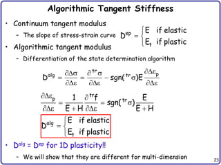
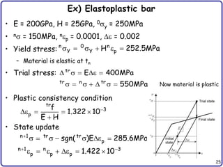
44. 44
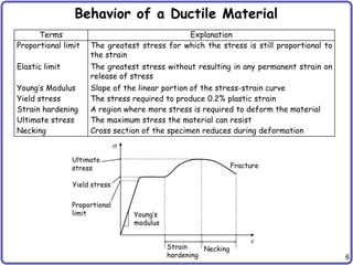
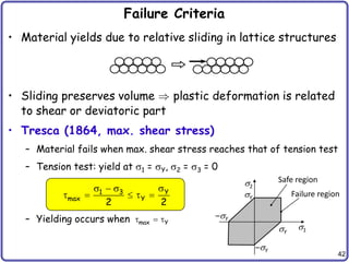
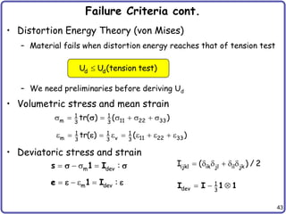
Failure Criteria cont.
• Example: Linear elastic material
• Distortion energy density
[ 2 ] : :
     
1 1 I D
s e e
m m
m
(3 ) 2 ( )
(3 2 ) 2
deviatoric
volumetric
s   e    e
    e  
1 e 1
1 e
m m
(3 2 )
2
s     e
 
s e
1 1
d 2 4
U : :

 
s e s s
3
1 1 1
m m m m
2 2 2 2
U : ( ) : ( ) :
  s  e   s e 
1 s 1 e s e
s e
Bulk modulus
3 2
K
3
  


45. 45
Failure Criteria cont.
• 1D Case
• Material yields when
• Let’s define an equivalent stress
• Then, material yields when
• Stress can increase from zero to sY, but cannot
increase beyond that
2
3
1 1
11 m 3 3
1
3
0 0
0 0
0 0
 
 
s  s s  s  s 
 
 

 
s
2 2
1 1 2 1
d 4 4 3 6
1D
U :
  
  s  s
s s
2
1 1
d Y d
4 6 1D
U : U
 
  s 
s s
3
e 2
:
s  s s
e Y
s  s
von Mises stress

46. 46
Equivalent Stress and Effective Strain
• Equivalent stress is the scalar measure of 3D stress state
that can be compared with 1D stress from tension test
• Effective strain is the scalar measure of 3D strain state
that makes conjugate with equivalent stress
1 1
d e e
2 2
U : e
  s
s e
2
1 1 1
d e e e
4 6 2
U : e
 
  s  s
s s
3 3
1 1 1 2
e e
3 3 2 3 2 3
e : 2 : 2 :
  
 s     
s s e e e e
Effective strain

47. 47
Equivalent Stress and Effective Strain cont.
• 1D Case cont.
2 0 0
(1 )
0 1 0
3
0 0 1
 
  e  
 
 
 

 
e
2
(1 )
: 6
3
  e
 
  
 
e e
2
e 3
2(1 )
e :
3
 
  e
e e Effective strain for 1D tension
11 22 33 m
1 2
3
 
e  e e  e  e e  e
ε ε

48. 48
Von Mises Criterion
• Material yields when se = sY
• Yield criterion
– 1D test data sY can be used for
multi-dimensional stress state
– Often called J2 plasticity model
3
e 2
2
: 3J
s  
s s
1
2 2
J :
 s s
2nd invariant of s
2 2 2
e Y 2 Y
3J 0
s  s   s 
2 2 2 2 2 2
2 x y y z z x xy yz zx
1
J ( ) ( ) ( )
6
 
 s  s  s  s  s  s      
 
2 2 2
2 1 2 2 3 3 1
1
J ( ) ( ) ( )
6
 
 s  s  s  s  s  s
 
σ1
σ2
Yield surface
Elastic 2
2
1
3
s
 Y
J
2
2
1
3
s
 Y
J

49. 49
Von Mises Criterion cont.
• J2: second invariant of s
• Von Mises yield function
2
1 1
2 2 2
J [ : tr( ) ] :
  
s s s s s
2
2 Y
3J 0
 s 
2
3
Y
2
: 0
  s 
s s
2
Y
3
: 0
  s 
s s
2
Y
3
0
  s 
s
Yield function
s1
s2
2
Y
3
 s
s
radius
Elastic
state
Impossible
state
Material
yields
Yield surface is circular in
deviatoric stress space

50. 50
Example
• Pure shear stress  to yield
– Yield surface:
– Failure in max. shear stress theory
Safe in distortion energy theory
– Von Mises is more accurate, but
Tresca is more conservative
0 0
0 0
0 0 0

 
 
  
 
 
 
σ s
2 2
: 2
      
s s s
2
Y Y
3
1
2
3
  s    s
s1
s2
D
C
Safe region
x1
x2
τ
τ
τ
τ

51. 51
Example
• Uniaxial tensile test
– Yield surface
2
3
1
3
1
3
0 0
0 0
0 0 0 0 0
0 0 0 0 0
 
s
s
 
 
 
   s
 
 
 
   s
   
s
s
2 2 2
4 1 1 2
9 9 9 3
 s  s  s  s
s
2 2
Y Y
3 3
0
s  s   s  s
s s
Consistent with uniaxial
tension test

52. 52
Hardening Model
• For many materials, the yield surface increases
proportional to plastic deformation strain hardening
• Isotropic hardening: Change in radius
• Kinematic hardening: Change in center
σ1
σ2
Initial yield surface
Isotropic hardening
σ1
σ2
Initial yield surface
Kinematic hardening

53. 53
Hardening Model cont.
• Isotropic hardening model (linear)
– H = 0: elasto-perfectly-plastic material
• Kinematic hardening model (linear)
– The center of yield surface : back stress 
– Shifted stress:  = s – 
–  moves proportional to ep
0
Y Y p
He
s  s 
p
p
0
Y
H Plastic modulus
e
e Effective plastic strain
Initial yield stress
s


s
2
Y
3
0
 s 

2
p
3
He




s1
s2
s
Radial
direction

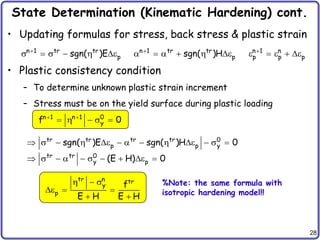
54. 54
Hardening Model cont.
• Combined Hardening
– Many materials show both isotropic and kinematic hardenings
– Introduce a parameter  [0, 1] to consider this effect
– Baushinger effect: The yield stress increases in one directional
loading. But it decreases in the opposite directional load.
– This is caused by dislocation pileups and tangles (back stress).
When strain direction is changed, this makes the dislocations easy
to move
– Isotropic hardening:  = 0
– Kinematic hardening:  = 1
0
2
Y p
3
[ (1 )He ] 0
 s    

2
p
3
He
 




55. 55
Rate-Independent Elastoplasticity
• Additive decomposition
• Strain energy (linear elastic)
• Stress (differentiating W w.r.t. strain)
p p
e e
   
e e e e e e From small deformation assumption
p p
e e e
1 1
2 2
W( ) : : ( ) : : ( )
   
D D
e e e e e e e
p
e
e
W
: : ( )

   

D D
s e e e
e
p
: ( )
 
D
s e e
2
    
D 1 1 I
2
dev
3
( ) 2
      
D 1 1 I
Why we separate volumetric part
from deviatoric part?

56. 56
Rate-Independent Elastoplasticity cont.
• Stress cont.
– Volumetric stress:
– Deviatoric stress:
• Yield function
– We will use von Mises, pressure insensitive yield function
– k(ep): Radius of elastic domain
– ep: effective plastic strain
• Elastic domain (smooth, convex)
1 2
m m
3 3
tr( ) ( )tr( ) (3 2 )
s          e
s e
p
2 ( )
  
s e e Why isn’t this
an elastic strain?
2
p p
3
f( ,e ) (e ) 0
  k 
 
 
p p
E ( ,e ) f( ,e ) 0
 
 
sn
str
sn+1
E, f<0
sn sn+1
str

57. 57
Rate-Independent Elastoplasticity cont.
• Flow rule (determine evolution of plastic strain)
– Plastic consistency parameter g : g > 0 (plastic), g =0 (elastic)
• Flow potential g(s, x)
– Plastic strain increases in the normal direction to the flow
potential
p
( , )
 gr
e s x p
( ,e )

x 
Plastic variables
p
g( , ) g( , )
 
   g
 
r
s x s x
e
s s
g1
g2
g3
g

s

58. 58
Rate-Independent Elastoplasticity cont.
• Associative flow rule
– Flow potential = yield function
p f( , )

 g

 x
e

f :
:

 
    
  
N
    
   
 
Unit deviatoric tensor
normal to the yield surface
p f

  g  g  g

N

e
 
N determines the direction of plastic strain rate
and determines the magnitude
g

59. 59
Rate-Independent Elastoplasticity cont.
• Evolution of plastic variables (hardening model)
• Back stress 
• Effective plastic strain
– Note: plastic deformation only occurs in deviatoric components
p
p p
f( ,e )
H (e ) H (e )
 

 g  g

N



Plastic modulus for
kinematic hardening
p p p p
2 2
3 3
e :
 
e e e
p p
 e
e
p
 g  g
N
e
p 2
3
e  g
p
( ,e )

x 
( , )
  gh
x s x

60. 60
Rate-Independent Elastoplasticity cont.
• Kuhn-Tucker conditions
– The plastic consistency parameter must satisfy
1. Within elastic domain:
2. On the yield surface
a. Elastic unloading
b. Neutral loading
c. Plastic loading (process attempt to violate f ≤ 0)
0 f 0 f 0
g  g  
f 0 0 f 0
 g   g 
f 0 0 f 0
 g   g 
f 0 0 f 0
 g   g 
f 0 0 f 0
 g   g 
f = 0
f = 0
Equivalent to f 0
g 

61. 61
Classical Elastoplasticity
• Elastoplasticity boils down to how to calculate plasticity
consistency parameter
• Classical plasticity uses the rate form of evolution
relations to calculate it
• Plastic consistency condition
– is only non-zero when continues plastic deformation
f 0
g 
g
0 f( , ) 0
g  
s x
f f
f( , ) : 0
 
   
 
s x s x
s x
p
f f
: : ( ) 0
 
   g 
 
D h
e e
s x
f f f
: : : : 0
  
 g   g 
  
D D r h
e
s s x
Solve for plastic
consistency parameter

62. 62
Classical Elastoplasticity cont.
f
: :
f f
: :


g 
 
 
 
D
D r h
e
s
s x
Assume the denominator is positive
x if x 0
x
0 if x 0


 


f
0 : : 0

g   

D e
s
E
: trial stress rate
D e
normal
f

s
q
f
: :
cos
f
:


q 


D
D
e
s
e
s
• Plastic consistency parameter
q < 90o : plastic loading
q = 90o : neutral loading
q > 90o : elastic unloading

63. 63
Classical Elastoplasticity cont.
• Elastoplastic tangent stiffness (when > 0)
p
: ( )
 
D
s e e
g
f
f f
: :
: : : :
: :


 
 
  g  
 
D
D D r D D r
D r h
s
s x
e
s e e
f
f f
: :
:
: :


 
 
 

 
 
 
 
 
D r D
D
D r h
s
s x
s e
f
ep
f f
: :
: :


 
 

 
 
D r D
D D
D r h
s
s x
Elastoplastic tangent operator
In general, it is not symmetric, but for associative flow rule, it is

64. 64
Nonlinear Hardening Models
• Nonlinear kinematic hardening model
• Nonlinear isotropic hardening model
p
p
p p 0
p
e
H(e ) H(e ) H exp
e
 
 
  
 
 
e
 Saturated hardening
0 0
p Y Y Y p p
(e ) ( ) 1 exp( e / e )
 
 
k  s  s  s  
 

65. 65
Example: Linear hardening model
• Linear combined hardening model, associative flow rule
• 5 params: 2 elastic (, ) and 3 plastic (, H, sY
0) variables
• Plastic consistency parameter
k  s      p
0 2
p Y p 3
(e ) (1 )He He

   s    
0
2
p Y p
3
f( , ,e ) [ (1 )He ] 0
s s
 
  
        
  
2
p p
3
p
f f f
f : : e : : (1 )He 0
e
s N s N
s
 

 
      g
    g
 g

p
p
2 2
3 3
2
p 3
2 2 2
H H
e
s e e e N
e N

66. 66
Example: Linear hardening model cont.
• Plastic consistency parameter cont.
– No iteration is required
• Elastoplastic tangent stiffness
   g   g    g 
2 2
3 3
f 2 : 2 : H : (1 )H 0
N N N N N
e


: 1
: :
N N
N e N e

g 
  2
3
2 :
2 H
N e
    g
p
: : : :
D D D D N
s e e e       
2
dev
3
( ) 2
D 1 1 I
 
: 2
D N N
 
 
     
 
   
 
 
2
2 2
3 3
2 : 4
: 2 :
2 H 2 H
N
D N D N N
e
s e e
Dep

67. 67
Numerical Integration
• Plastic evolution is given in the rate form
• We will use backward Euler method to integrate it
• Assumptions
– We assume that all variables are known at load step n:
– At the current time n+1, is given
• We will use 2-step procedure
1. Predictor: elastic trial
2. Corrector: plastic return mapping (projection onto the yield
surface)
n 1 n
n 1 n 1
y y
y f(t, y) f(t y )
t

 

  

n 1 n n 1 n 1
y y t f(t y )
  
     A-stable
Stable for all t
,
n n
s x
or
 
u e

68. 68
Numerical Integration cont.
1. Elastic predictor
– Shifted stress:
– Yield function:
2. Plastic corrector
1. If f < 0 (within the elastic domain)
– Exit
tr n tr n tr n
p p
2 e e
    
s s e  
No plasticity
dev. inc. strain
tr tr tr
 
s
 
tr n tr n
2
p p
3
f( ,e ) (e )
  k
 
n 1 tr n 1 tr n 1 tr
p p
e e
  
 
s s   

69. 69
Numerical Integration cont.
2. Plastic corrector cont.
2. If f > 0 (return mapping to yield surface)
• Trial direction is parallel to final direction
n 1 tr
p
2

   
s s e p
e  gN
unknown
n 1 tr
2

  g
s s N
n 1 tr
H


  gN
 
n 1 n 1 n 1 tr
(2 H )
  

      g
s N
  
So far, unknowns are n 1 n 1
and  
g 
N  
  
   
     
n 1 tr n 1 tr n 1
n 1 tr
n 1 tr


 
N
 
 
Known from trial state

70. 70
Numerical Integration cont.
2. Plastic corrector cont.
– Now the plastic consistency parameter is only unknown!!
– How to compute: stress must stay on the yield surface
– While projecting the trial stress,
the yield surface also varies
– But, both happen in the same
direction N
n 1 n 1
p
f( ,e ) 0
 


sn
str
sn+1
n
n+1
n 1 n 1
p
f( ,e ) 0
 


n n
p
f( ,e ) 0


   
  k 
 
n 1 n 1 n 1 n 1
2
p p
3
f( ,e ) (e ) 0
n 1 tr tr
(2 H ) (2 H )

 
    g     g
N
  

71. 71
Numerical Integration cont.
2. Plastic corrector cont.
– Plastic consistency condition
– Nonlinear (scalar) equation w.r.t. g
– Use Newton-Raphson method (start with )
– Stop when f ~ 0
 
tr n 1 n 1
2
p p
3
2 H (e ) (e ) 0
 

   g  k 

n 1 n 2
p p 3
e e

  g


k
     g 
g
2 2
3 3
p p
dH
df d
(2 H )
d de de
 
 

    g  k
tr n 1 n 1
2
p p
3
f 2 H (e ) (e )
g  g 
g
f
df / d
 
  g
n 1 n 1 2
p p 3
e e

g  
n 1 n
p p
0, e e

72. 72
Numerical Integration cont.
• When N-R iteration is converged, update stress
n 1 n
2 2

    g
s s e N
n 1 n
: 2

    g
D N
s s e
n 1 n
H


  gN
 
n 1 n 2
p p 3
e e

  g
Tangent operator
ep
: 
D e

73. 73
Consistent Tangent Operator
• Consistent tangent operator – tangent operator that is
consistent with numerical integration algorithm
• Differentiate stress update equation
ep alg
 
 
 
D D
s s
e e
: 2
    g
D N
s e
2 2
 g 
     g
  
N
D N
s
e e e
(1) (2)
Continuum tangent operator Consistent tangent operator

74. 74
Consistent Tangent Operator cont
• Term (1) n 1 n 1 n n
p p
f( ,e ) f( ,e ) 0
 
 
 
f
0

 
e
 

   
    g  k 
 
 

e e
tr n 1 n 1
2
p p
3
f
(2 H (e )) (e ) 0
tr tr tr 1/2 tr
tr
tr
( : ) 1 1
2 :
2
  
 
  
   

e e e

tr tr tr
tr
: 2
 
  
 
N
  
e e

tr tr n
dev
( )
2
 
  
 
s
I
  
e e
p p
n 1 2
p 3
p p
e e
H
f
2 (2 H (e )) 0
e e
 

 

 g k
      g  
     
N
e e e e
 

 
g
     g  k 
e
p p
n 1 2 2
p ,e ,e
3 3
2 2 H (e ) H 0
N
2
3
g
e
2 A
g
 

N
e

 
    g  k
p p
n 1 2 2
p ,e ,e
3 3
1
2 H (e ) H
A

75. 75
Consistent Tangent Operator cont
• Term (2):
• Consistent tangent operator
tr
tr
:
  

 

N N 
e e

tr
n n
dev
( 2 ) 2
 
     
 
s e I


e e
 
   
 
     
 
 
 
  
 
  
    

tr tr tr
tr tr tr tr 3 tr
tr
1
N I
I N N
dev dev
tr tr
1 2
: 2
 
      
   
   

N
I N N I I N N
e  
alg
dev
tr
2
2 (2 A ) 2
 
       g  
 
 

D D N N I N N
s
e 
2
alg 2
dev
tr
4
4 A
 g
      
 
 
D D N N I N N

Not existing in Dep

76. 76
Example
• Linear combined hardening
• Consistency condition
p
n 1 2
p ,e
3
n 1 0 n 1 n 2
p Y p p 3
H (e ) H H 0
(e ) (1 )He (e ) (1 )H

 
 
  
k  s     k    g
   
tr n
2 2 2
p
3 3 3
f 2 H (e ) (1 )H 0
     g  k    g 

tr n
2
p
3
2
3
(e )
2 H
 k
 g 
 

No iteration is required
1 2
2 H
A 3
  

77. 77
Variational Equation
• Variational equation
– The only nonlinearity is from stress (material nonlinearity)
– Small strain, small rotation
• Linearization
• Update displacement
n n 1 n 1
a( ; , ) ( ) : d
 

 

u u u
x e s
n n 1
a( ; , ) ( ),

  
u u u u
x
alg
* n n 1
a ( , ; , ) ( ) : : ( ) d .


   

u u u u D u
x e e
* n n 1 k k n n 1 k
a ( , ; , ) ( ) a( ; , ), ,
 
    
u u u u u u u
x x
n 1 k 1 n 1 k k
  
  
u u u

78. 78
Implementation of Elastoplasticity
• We will explain for a 3D solid element at a Gauss point
• Voigt notation
• Inputs
(a) Finite Element (b) Reference Element
x

z
(1,1,–1)
(1,1,1)
(–1,1,1)
(–1,1,–1)
x1
x2
x3
x4
x5
x6
x7
x8
x2
x1
x3
(1, –1,–1)
(1, –1,1)
(–1, –1,1)
T
11 22 33 12 23 13
{ } [ ]
 s s s s s s
s
T
11 22 33 12 23 13
{ } [ 2 2 2 ]
  e e e e e e
e
 
T
I I1 I2 I3
d d d
    
d
 
T
n n n n n n n
11 22 33 12 23 13
 s s s s s s
s
 
T
n n n n n n n n
11 22 33 12 23 13 p
e
      
x

79. 79
Implementation of Elastoplasticity cont.
• Displacement
x = {x, , z}T is the natural coordinates at an integration point
• Strain
• Update
8
I I
I 1

  
B u
e
8
I I
I 1
N ( )

  

u d
x
I,1
I,2
I,3
I
I,2 I,1
I,3 I,2
I,3 I,1
N 0 0
0 N 0
0 0 N
N N 0
0 N N
N 0 N
 
 
 
 
 

 
 
 
 
 
B
n 1 n

  
u u u
n 1 n
{ } { } { }

  
e e e

80. 80
Return Mapping Algorithm
• Elastic predictor
– Unit tensor
– Trial stress
– Trace of stress
– Shifted stress
– Norm
– Yield function
T
1 1 1 0 0 0
  
 
1
tr n
   
C
s s e
tr tr tr
11 22 33
tr( )  s  s  s
s
tr tr n
1
3
tr( )
  
 s s 
tr tr 2 tr 2 tr 2 tr 2 tr 2 tr 2
11 22 33 12 23 13
( ) ( ) ( ) 2[( ) ( ) ( ) ]
           

tr 0 n
2
Y p
3
f (1 )He
 
  s   
 


81. 81
Return Mapping Algorithm cont.
• Check yield status
– If f < 0, then the material is elastic
– Exit
• Consistency parameter
• Unit deviatoric tensor
• Update stress
• Update back stress
• Update plastic strain
• Calculate consistent tangent matrix
alg
n 1 tr

 
D D
s s
2
3
f (2 H)
g   
tr tr

N  
n 1 tr
2

  gN
s s
n 1 n 2
3
H

   gN
 
n 1 n 2
p p 3
e e

  g

82. 82
Implementation of Elastoplasticity cont.
• Consistent tangent matrix
• Internal force and tangent stiffness matrix
• Solve for incremental displacement
• The algorithm repeats until the residual reduces to zero
• Once the solution converges, save stress and plastic
variables and move to next load step
2 2
1 2
2 tr
3
4 4
c c
2 H
  g
 
  
alg T
1 2 2 dev
(c c ) c
   
D D NN I
ext int
T
[ ]{ } { } { }
  
K u f f
4 NG
int T n 1
I K K
I 1K 1
( )

 
 

f B J
s
4 4 NG
alg
T
T I J K K
I 1 J 1K 1
( )
  
 
  
K B D B J
2 1 1
3 3 3
1 2 1
3 3 3
1 1 2
dev 3 3 3
1
2
1
2
1
2
0 0 0
0 0 0
0 0 0
0 0 0 0 0
0 0 0 0 0
0 0 0 0 0
 
 
 
 
 
 
 
 

 
 
 
 
 
I

83. 83
Program combHard.m
%
% Linear combined isotropic/kinematic hardening model
%
function [stress, alpha, ep]=combHard(mp,D,deps,stressN,alphaN,epN)
% Inputs:
% mp = [lambda, mu, beta, H, Y0];
% D = elastic stiffness matrix
% stressN = [s11, s22, s33, t12, t23, t13];
% alphaN = [a11, a22, a33, a12, a23, a13];
%
Iden = [1 1 1 0 0 0]';
two3 = 2/3; stwo3=sqrt(two3); %constants
mu=mp(2); beta=mp(3); H=mp(4); Y0=mp(5); %material properties
ftol = Y0*1E-6; %tolerance for yield
%
stresstr = stressN + D*deps; %trial stress
I1 = sum(stresstr(1:3)); %trace(stresstr)
str = stresstr - I1*Iden/3; %deviatoric stress
eta = str - alphaN; %shifted stress
etat = sqrt(eta(1)^2 + eta(2)^2 + eta(3)^2 ...
+ 2*(eta(4)^2 + eta(5)^2 + eta(6)^2));%norm of eta
fyld = etat - stwo3*(Y0+(1-beta)*H*epN); %trial yield function
if fyld < ftol %yield test
stress = stresstr; alpha = alphaN; ep = epN;%trial states are final
return;
else
gamma = fyld/(2*mu + two3*H); %plastic consistency param
ep = epN + gamma*stwo3; %updated eff. plastic strain
end
N = eta/etat; %unit vector normal to f
stress = stresstr - 2*mu*gamma*N; %updated stress
alpha = alphaN + two3*beta*H*gamma*N; %updated back stress

84. 84
Program combHardTan.m
function [Dtan]=combHardTan(mp,D,deps,stressN,alphaN,epN)
% Inputs:
% mp = [lambda, mu, beta, H, Y0];
% D = elastic stiffness matrix
% stressN = [s11, s22, s33, t12, t23, t13];
% alphaN = [a11, a22, a33, a12, a23, a13];
%
Iden = [1 1 1 0 0 0]';
two3 = 2/3; stwo3=sqrt(two3); %constants
mu=mp(2); beta=mp(3); H=mp(4); Y0=mp(5); %material properties
ftol = Y0*1E-6; %tolerance for yield
stresstr = stressN + D*deps; %trial stress
I1 = sum(stresstr(1:3)); %trace(stresstr)
str = stresstr - I1*Iden/3; %deviatoric stress
eta = str - alphaN; %shifted stress
etat = sqrt(eta(1)^2 + eta(2)^2 + eta(3)^2 ...
+ 2*(eta(4)^2 + eta(5)^2 + eta(6)^2));%norm of eta
fyld = etat - stwo3*(Y0+(1-beta)*H*epN); %trial yield function
if fyld < ftol %yield test
Dtan = D; return; %elastic
end
gamma = fyld/(2*mu + two3*H); %plastic consistency param
N = eta/etat; %unit vector normal to f
var1 = 4*mu^2/(2*mu+two3*H);
var2 = 4*mu^2*gamma/etat; %coefficients
Dtan = D - (var1-var2)*N*N' + var2*Iden*Iden'/3;%tangent stiffness
Dtan(1,1) = Dtan(1,1) - var2; %contr. from 4th-order I
Dtan(2,2) = Dtan(2,2) - var2;
Dtan(3,3) = Dtan(3,3) - var2;
Dtan(4,4) = Dtan(4,4) - .5*var2;
Dtan(5,5) = Dtan(5,5) - .5*var2;
Dtan(6,6) = Dtan(6,6) - .5*var2;

85. 85
Program PLAST3D.m
function PLAST3D(MID, PROP, ETAN, UPDATE, LTAN, NE, NDOF, XYZ, LE)
%***********************************************************************
% MAIN PROGRAM COMPUTING GLOBAL STIFFNESS MATRIX RESIDUAL FORCE FOR
% PLASTIC MATERIAL MODELS
%***********************************************************************
%%
....
%LOOP OVER ELEMENTS, THIS IS MAIN LOOP TO COMPUTE K AND F
for IE=1:NE
DSP=DISPTD(IDOF);
DSPD=DISPDD(IDOF);
%....
% LOOP OVER INTEGRATION POINTS
for LX=1:2, for LY=1:2, for LZ=1:2
%
% Previous converged history variables
NALPHA=6;
STRESSN=SIGMA(1:6,INTN);
ALPHAN=XQ(1:NALPHA,INTN);
EPN=XQ(NALPHA+1,INTN);
....
% Computer stress, back stress & effective plastic strain
if MID == 1
% Infinitesimal plasticity
[STRESS, ALPHA, EP]=combHard(PROP,ETAN,DDEPS,STRESSN,ALPHAN,EPN);
....
%
% Tangent stiffness
if LTAN
if MID == 1
DTAN=combHardTan(PROP,ETAN,DDEPS,STRESSN,ALPHAN,EPN);
EKF = BM'*DTAN*BM;
....

86. 86
Summary
• 1D tension test data are used for 2D or 3D stress state
using failure theories
– All failure criteria are independent of coordinate system (must
defined using invariants)
• Yielding of a ductile material is related to shear stress or
deviatoric stress
• Kinematic hardening shift the center of elastic domain,
while isotropic hardening increase the radius of it
• For rate-independent J2 plasticity, elastic predictor and
plastic correct algorithm is used
• Return mapping occurs in the radial direction of deviatoric
stress
• During return mapping, the yield surface also changes

87. 87
Elastoplasticity with Finite
Rotation
Section 4.4

88. 88
Goals
• Understand the concept of objective rate and frame-
indifference (why do we need objectivity?)
• Learn how to make a non-objective rate to objective one
• Learn different objective stress rates
• Learn how to maintain objectivity at finite rotation
• Understand midpoint configuration
• Understand how to linearize the energy form in the
updated Lagrangian formulation
• Understand how to implement update Lagrangian frame

89. 89
Elastoplasticity with Finite Rotation
• We studied elastoplasticity with infinitesimal deformation
– Infinitesimal deformation means both strain and rotation are small
• We can relax this limitation by allowing finite rotation
• However, the engineering strain changes in rigid-body
rotation (We showed in Chapter 3)
• How can we use engineering strain
for a finite rotation problem?
• Instead of using X, we can use xn as a reference
(Body-fixed coordinate, not Eulerian but Lagrangian)
• Can the frame of reference move?
rotation
strain
sym( ) skew( )
    
u u u
cos 1 0 0
0 cos 1 0
0 0 0
 
 
 
  
 
 
 
e

90. 90
Objective Tensor
• We want to take care of the issues related to the moving
reference frame xn (rotation and translation) using
objectivity
• Objective tensor: any tensor that is not affected by
superimposed rigid body translations and rotations of the
spatial frame
• Rotation of a body is equivalent to rotation of coordinate
frame in opposite direction
• Consider two frames in the figure
(rotation + translation)
x
P
x
 
x y z
 
x y z
(t) (t)
  
x Q x c
x and are different by rigid-body motion,
by relative motion between observers
x

91. 91
Objective Tensor cont.
• Frame indifference (objectivity)
– Quantities that depend only on Q and not on the other aspects of
the motion of the reference frame (e.g., translation, velocity and
acceleration, angular velocity and angular acceleration)
• Objective scalar
• Objective vector
• Objective tensor
• In order to use a moving reference, we must use
objective quantities
f f

 
v Q v
T
  
T Q T Q

92. 92
Example
• Deformation gradient
– F transforms like a vector
• Right C-G deformation tensor
– Material tensors are not affected by rigid-body motion
• Left C-G deformation tensor
• Objectivity only applies to a spatial tensor, not
material tensor
• Deformation gradient transforms like a vector because it
has one spatial component and one material component
( (t) (t)) (t) (t)
  
       
  
x x
F Q x c Q Q F
X X X
T T T T T
( ) ( )
    
C F F QF QF F Q QF F F C
T T T T T T
( )( )
   
b FF QF F Q QFF Q QbQ
Objective
tensor

93. 93
Velocity Gradient
• In two different frames
• Time differentiate of
• Spatial differentiation of
,
 
 
 
v v
L L
x x
 
x Q x
   
x Q v Q x
T
  
v Q v QQ x Velocity is not objective
v
T
T T



  
     
  
    
v
L
x
v x x
Q Q Q
x x x
Q L Q Q Q
Velocity gradient is not objective
Velocity gradient is related to incremental
displacement gradient in finite time step
t

 

u
L
x

94. 94
Rate of Deformation and Spin Tensor
• Rate of Deformation
• Spin tensor
sym( ) sym( )
 
d L d L
 
T T T T T
1
2
sym( )
          
d L Q L Q Q L Q Q Q Q Q
T T T
      
Q Q 1 Q Q Q Q 0
T T T
1
2
( )
      
d Q L L Q Q d Q Objective
This is incremental stain
T T
1 1
2 2
( ) ( )
   
W L L W L L
T T T T T T
1 1
2 2
( ) ( )
           
W L L Q L Q Q L Q Q Q Q Q
T T T
1
2
( )
      
W Q W Q Q Q Q Q
Not Objective
Depends on the spin of rotating frame

95. 95
Cauchy Stress Is an Objective Tensor
• Proof from the relation between stresses
• Proof from coordinate transformation of stress tensor
– Coordinate transformation is opposite to rotation

s T
1
J
FSF

S S
 
   
 
 
s s
T T T T T T
1 1 1
J J J
FSF QFSF Q Q FSF Q Q Q
x
y
z
x
y
z
b1
b2
b3
 
s s
1 2 3
( ) ( ) ( ) 1 2 3
xyz xyz xyz
[ ] [ ] [ ] [ ] [ ]
b b b
T T T b b b Q
   
s s
T
x y z xyz
[ ] [ ] [ ] [ ]
Q Q

s s T
xyz xyz
[ ] [ ][ ] [ ]
Q Q

96. 96
Objective Rate
• If T is an objective tensor, will its rate be objective, too?
– This is important because in plasticity the constitutive relation is
given in terms of stress rate
• Differentiate an objective tensor
– Not objective due to
• Remove non-objective terms using
T
  
T Q T Q
T T T
        
T Q T Q Q T Q Q T Q
and T
Q Q
T T
    
L Q L Q Q Q
T T T T T
       
Q L Q Q L Q Q L L Q
T T T T T T
T T T T T T T
T T T T T
( ) ( )
    
    
    
T LQ QL TQ QTQ QT Q L L Q
LQTQ QLTQ QTQ QTQ L QTL Q
LT QLTQ QTQ TL QTL Q

97. 97
Objective Rate cont.
• Objective rate
• Thus, is an objective rate (Truesdell rate)
• Co-rotational rate (Jaumann rate)
• Convected rate
• These objective rates are different, but perform equally
• When T is stress, they are objective stress rate
T T T T T
    
T LT QLTQ QTQ TL QTL Q
T T T
( )
    
T LT TL Q T LT TL Q
T
 
T LT TL
   
T W T T W
T
   
T L T T L

98. 98
Finite Rotation and Objective Rate
• Since constitutive relation should be independent of the
reference frame, it has to be given in terms of
objective rate
• Cauchy stress is an objective tensor, but Cauchy stress
rate is not objective rate
• Instead of rate, we will use increment (from previous
converged load step to the current iteration)
• Consider a unit vector ej in spatial Cartesian coordinates
under rigid body rotation from material vector Ej
j j j j
        
e Q E W Q E W e
T
T
1
2
 
 
    
 
 
 
 
u u
W Q Q
x x
j j
 
e Q E
W: spin tensor
Q: rotation tensor

99. 99
Finite Rotation and Objective Rate cont.
• Cauchy stress in Cartesian coordinates
• Incremental Cauchy stress
• Constitutive relation
ij i j
 s 
e e
s
  s   s    s  
 s    s   s  
 s  s  s 
s ij i j ij i j ij i j
J T
ij i j ij i j ij i j
J
ij ik kj ik kj i j
( ) ( )
( W W )
e e e e e e
e e W e e e e W
e e
Jaumann or co-rotational Cauchy stress increment
Objective rate in the rotating frame
J
alg :
  
C
s e
Effect of rigid body rotation
Only accurate for small, rigid body rotations
J
    
W W
s s s s

100. 100
Finite Rotation and Objective Rate cont.
• For finite rotation, the spin tensor W is not constant
throughout the increment
• Preserving objectivity for large rotational increments
using midpoint configuration
• Instead of n+1, calculate strain increment and spin at n+½
• Midpoint configuration
– We want to rotation stress into the midpoint configuration
1 1
2 2
j
i
ij n n
j i
u
u
1
2 x x
 
 


 
e  
 
 
 
1 1
2 2
j
i
ij n n
j i
u
u
1
W
2 x x
 
 


 
 
 
 
 
1
2
n n 1 n n n 1
1 1 1
2 2 2
( )
  
       
x x x x u x u
How to calculate these?
n 1 2
n
n 1 2 n n 1 2 n n
1
,
2

 
    
   
  
 
u u x x u
1
x x x
x x

101. 101
Finite Rotation and Objective Rate cont.
• Rotational matrix to the midpoint configuration
• Rotation of stress and back stress
• Now, return mapping with these stresses
– Exactly same as small deformation plasticity
n n T
n n T
  
  
R R
R R
s s
 
d
dt
 
R
W R
1 1
1 1 1
2 2 2
( ) ( ) ( )
 
      
R 1 W 1 W 1 1 W W
1
2
n 1 n n 1 n
n
( ) ( )
t 2
 

 
   

R R R R
W u R W u
( ) t ( )
  
W u W u
n 
R 1
This takes care of rigid body rotation

102. 102
Program rotatedStress.m
%
% Rotate stress and back stress to the rotation-free configuration
%
function [stress, alpha] = rotatedStress(L, S, A)
%L = [dui/dxj] velocity gradient
%
str=[S(1) S(4) S(6);S(4) S(2) S(5);S(6) S(5) S(3)];
alp=[A(1) A(4) A(6);A(4) A(2) A(5);A(6) A(5) A(3)];
factor=0.5;
R = L*inv(eye(3) + factor*L);
W = .5*(R-R');
R = eye(3) + inv(eye(3) - factor*W)*W;
str = R*str*R';
alp = R*alp*R';
stress=[str(1,1) str(2,2) str(3,3) str(1,2) str(2,3) str(1,3)]';
alpha =[alp(1,1) alp(2,2) alp(3,3) alp(1,2) alp(2,3) alp(1,3)]';

103. 103
Variational Principle for Finite Rotation
• Total Lagrangian is inconvenient
– We don’t know how 2nd P-K stress evolves in plasticity
– plastic variables is directly related to the Cauchy stress
• Thus, we will use the updated Lagrangian formulation
• Assume the problem has been solved up to n load step, and
we are looking for the solution at load step n+1
• Since load form is straightforward, we will ignore it
• Energy form
– Since the Cauchy stress is symmetric, it is OK to use
– Both n+1 and sn+1 are unknown
– Nonlinear in terms of u
n 1

 u
n 1
n n 1 n 1
n 1
a( ; , ) : d

 


  

u u u
x s

104. 104
Variational Principle for Finite Rotation cont.
• Energy form cont.
– Since the current configuration is unknown (depends on displace-
ment) , let’s transform it to the undeformed configuration 0
– Integral domain can be changed by
– This is only for convenience in linearization. Eventually, we will
come back to the deformed configuration and integrate at there
– The integrand is identical to where is the
first P-K stress
– Nonlinearity comes from (a) constitutive relation (hypoelasticity),
(b) spatial gradient (deformation gradient), and (c) Jacobian of
deformation gradient (domain change)
n 1 0
n n 1 n 1 1 n 1
n 1 0
a( ; , ) : d ( ) : Jd

   

 
     
 
u u u uF
x s s
:
T F 1
J 

T F s
n 1 0
d Jd J det( )

 
   
  F

105. 105
Linearization
• Increment of deformation gradient
• Increment of Jacobian
0
0
( )

    
 
     
 
  
 
x u u
F u
X X
1 1 1 1 1
0 n 1
    

          
FF 1 F F uF F u
J Jdiv( )
    
F u
1
mn ijk rst ir js kt
6
F e e F F F

ijk ijr kr
e e 2
 

106. 106
Linearization cont.
• Linearization of energy form
0
0
0
n 1
1
0
1 1 1
0 0 0
1 1 1
0 n 1 0 0
n 1 n 1 n 1 n 1
T
n 1 n 1
( ) : Jd
( ) : J ( ) : J ( ) : J d
: : : div( ) Jd
: : : div( ) d
: div( ) ( )



  

  


   

 
  
 
         
 
 
          
 
          
 
 
       




uF
u F uF uF
uF u uF uF u
u u u u u
u u u
s
s s s
s s s
s s s
s s s
n 1
d


  
 

T
ik kj ij ik ij kj
: : A B C A C B
 
AB C A CB
Use Jaumann objective rate

107. 107
Linearization cont.
• Linearization of energy form cont.
– Express inside of [ ] in terms of
– Constitutive relation:
– Spin term
n 1
n 1
n n 1 T
n 1 n 1
J T
n 1 n 1
L[a( ; , )] : div( ) ( ) d
: div( ) ( ) d



 

 

 
        
 
 
          
 


u u u u u
u W W u u
x s s s
s s s s s
alg alg
J
n 1
: : ( )

    
D D u
s e 
n 1

 u
m k
i
m i l
u u
u
1 1
im mj mj mj ik ml mk il
2 x x 2 x
1
lj ik kj il n 1 kl
2
W ( ) ( )
( )[ ]
 

  

s   s  s     
 s   s   u
1
im mj il jk ik jl n 1 kl
2
W ( )[ ]

s  s   s   u
k
k
u
ij ij kl n 1 kl
x
[ ]



s  s   u
j
m
u
im il jk n 1 kl
x
[ ]



s  s   u

108. 108
Linearization cont.
• Linearization of energy form cont.
– Initial stiffness term (we need to separate this term)
– Define
n 1
J T
n 1 n 1
L[a( , )] : div( ) ( ) d

 

 
          
 

u u u W W u u
s s s s s
1
jl ik jk il il jk ik jl ij kl
2
( )
s   s   s   s   s 
m m m m k
i
r s r s j l
T
n 1 n 1
u u u u u
u
1
rs jl ik
2 x x x x x x
: sym( ) : ( , )
( )
 
    

     
    
s   s 
u u u u
s s 
* 1
ijkl ij kl il jk jl ik ik jl jk il
2
( )
  s   s   s   s   s 
D
Rotational effect of Cauchy stress tensor

109. 109
Linearization cont.
• Linearization of energy form cont.
• N-R iteration
* n n 1 n n 1
k k 1 k
a ( , ; , ) ( ) a( ; , ),
 

    
u u u u u u u
x x Z
n 1
alg
n n 1 *
n 1 n 1
* n n 1
L[a( ; , )] : ( ) : : ) d
a ( , ; , )


 


 
       
 
 

u u u D D u u u
u u u
x s  
x
Bilinear
History-dependent
(implicit)

110. 110
Implementation
• We will explain using a 3D solid element at a Gauss point
using updated Lagrangian form
• The return mapping and consistent tangent operator will
be the same with infinitesimal plasticity
• Voigt Notation
• Inputs
T
11 22 33 12 23 13
{ } [ ]
 s s s s s s
s
T
11 22 33 12 23 13
{ } [ 2 2 2 ]
  e e e e e e
e
 
T
I I1 I2 I3
d d d
    
d
 
T
n n n n n n n
11 22 33 12 23 13
 s s s s s s
s
 
T
n n n n n n n n
11 22 33 12 23 13 p
e
      
x

111. 111
Implementation cont.
• In the updated Lagrangian, the derivative is evaluated at
the current configuration (unknown yet)
• Let the current load step is n+1 (unknown) and k+1 N-R
iteration
• Then, we use the configuration at the previous iteration
(n+1, k) as a reference
• This is not ‘true’ updated Lagrangian, but when the N-R
iteration converges, k is almost identical to k+1
• Caution: we only update stresses at the converged load
step, not individual iteration
• All derivatives and integration in updated Lagrangian must
be evaluated at (n+1, k) configuration
• Displacement increment u is from (n+1,0) to (n+1,k)

112. 112
Implementation cont.
• Stress-displacement matrix (Two approaches)
1. Mapping between current (n+1, k) and reference configurations
2. Mapping between undeformed and reference configurations
3
1 2
3
1 2
3
1 2
x
x x
x
x x
x
x x

 
 
 
x x x
 

 
 
  
  
 

 
 
 
z z z
 
J
1
1
2
3
x
x
x

 
 
 
   
 x
   
 
   

   
 
   


   
   
z
  
 
J
1
n 1 0


  
u F u
Use this for B matrix
1 1
1
2 2
3 3
x X
x X
x X

   
 
   
 
   
 
   

   
 
   
 
   
   
 
   
F

113. 113
Implementation cont.
1. Obtain midpoint configuration (between k and k+1)
2. Rotation matrix:
3. Rotate stresses:
4. Return mapping with
– This part is identical to the classical return mapping
– Calculate stresses:
– Calculate consistent tangent operator Dalg
n
n 1 2 n n 1 2
 
  
 

 
u u x
x
x x
1
n
n 1 2 n
1
2


 
 
 
 

  
x u
1
x
x
1 1
2 2
n n
sym( ) skew( )
 
      
u W u
e
1
1
2
( )
  
R 1 1 W W
n n T n n T
     
R R R R
s s  
n n
,
s 
n 1 n 1
k 1 k 1
,
 
 
s 

114. 114
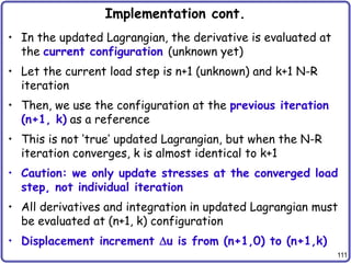
Implementation cont.
• Internal force
• Tangent stiffness matrix
• Initial stiffness matrix
4 NG
int T n 1
I k 1 K K
I 1K 1
( )


 
 

f B J
s
4 4 NG
alg
T *
T I J K K
I 1 J 1K 1
[ ( ) ]
  
  
  
K B D D B J
11 11 11 12 13
22 22 22 12 23
33 33 33 23 13
*
1 1 1
12 12 11 22 13 23
2 2 2
1 1 1
23 23 13 22 33 12
2 2 2
1 1 1
13 13 23 12 11 33
2 2 2
0
0
0
0 ( )
0 ( )
0 ( )
s s s s s
 
 
s s s s s
 
 
s s s s s
 

s s  s  s  s  s
 
 
s s  s  s  s  s
 
s s  s  s  s  s
 
 
D
T
4 4 NG
G G
S I J K K
I 1 J 1K 1
[ ]
  
 
  
K B B J

I,1
I,2
I,3
I,1
G
I,2
I
I,3
I,1
I,2
I,3
N 0 0
N 0 0
N 0 0
0 N 0
0 N 0
[ ]
0 N 0
0 0 N
0 0 N
0 0 N
 
 
 
 
 
 
 
  
 
 
 
 
 
 
 
B
9x9
[ ]
 
 
  
 
 
0 0
0 0
0 0
s
 s
s
This summation is similar to
assembly (must be added to the
corresponding DOFs)

115. 115
Implementation cont.
• Solve for incremental displacement
• Update displacements
• When N-R iteration converges
– Stress and history dependent variables are stored (updated) to
the global array
– Move on to the next load step
ext int
T S k 1
[ ]{ } { } { }

   
K K d f f
n 1 n 1
k 1 k k 1
k 1 k 1 k 1
 
 
  
  
    
d d d
d d d

116. 116
Program PLAST3D.m
function PLAST3D(MID, PROP, ETAN, UPDATE, LTAN, NE, NDOF, XYZ, LE)
%***********************************************************************
% MAIN PROGRAM COMPUTING GLOBAL STIFFNESS MATRIX RESIDUAL FORCE FOR
% PLASTIC MATERIAL MODELS
%***********************************************************************
....
% Computer stress, back stress & effective plastic strain
elseif MID == 2
% Plasticity with finite rotation
FAC=FAC*det(F);
[STRESSN, ALPHAN] = rotatedStress(DEPS, STRESSN, ALPHAN);
[STRESS, ALPHA, EP]=combHard(PROP,ETAN,DDEPS,STRESSN,ALPHAN,EPN);
....
%
% Tangent stiffness
if LTAN
elseif MID == 2
DTAN=combHardTan(PROP,ETAN,DDEPS,STRESSN,ALPHAN,EPN);
CTAN=[-STRESS(1) STRESS(1) STRESS(1) -STRESS(4) 0 -STRESS(6);
STRESS(2) -STRESS(2) STRESS(2) -STRESS(4) -STRESS(5) 0;
STRESS(3) STRESS(3) -STRESS(3) 0 -STRESS(5) -STRESS(6);
-STRESS(4) -STRESS(4) 0 -0.5*(STRESS(1)+STRESS(2)) -0.5*STRESS(6) -0.5*STRESS(5);
0 -STRESS(5) -STRESS(5) -0.5*STRESS(6) -0.5*(STRESS(2)+STRESS(3)) -0.5*STRESS(4);
-STRESS(6) 0 -STRESS(6) -0.5*STRESS(5) -0.5*STRESS(4) -0.5*(STRESS(1)+STRESS(3))];
SIG=[STRESS(1) STRESS(4) STRESS(6);
STRESS(4) STRESS(2) STRESS(5);
STRESS(6) STRESS(5) STRESS(3)];
SHEAD=zeros(9);
SHEAD(1:3,1:3)=SIG;
SHEAD(4:6,4:6)=SIG;
SHEAD(7:9,7:9)=SIG;
EKF = BM'*(DTAN+CTAN)*BM + BG'*SHEAD*BG;
....

117. 117
Summary
• Finite rotation elastoplasticity is formulated using
updated Lagrangian (reference frame moves with body)
• Finite rotation elastoplasticity is fundamentally identical
to the classical plasticity. Only rigid-body rotation is taken
into account using objective stress rate and integration
• We must use an objective stress rate to define the
constitutive relation because the material response should
be independent of coordinate system
• Objectivity only applies for spatial vectors and tensors
• In the finite rotation, the midpoint configuration is used
to reduce errors involved in non-uniform rotation and spin
• Linearization is performed after transforming to the
undeformed configuration

118. 118
Finite Deformation
Elastoplasticity with
Hyperelasticity
Section 4.5

119. 119
Goals
• Understand the difference between hypoelasticity and
hyperelasticity
• Learn the concept of multiplicative decomposition and
intermediate configuration
• Understand the principle of maximum dissipation
• Understand the plastic evolution in strain space and stress
space
• Learn J2 plasticity in principal stress space

120. 120
Finite Deformation Plasticity
• So far, we used small strain elastoplasticity theory
• Finite rotation has been taken care of using the deformed
configuration with an objective rate
• However, still, the strain should be small enough so that
the elastic and plastic strains are decomposed additively
• This is fundamental limitation of hypoelasticity
• How can we handle large strain problem?
• On the other hand, hyperelasticity can handle large strain
• However, it is not easy to describe plastic evolution in 2nd
P-K stress. It is given in the current configuration (Cauchy
stress)
• How can we handle it?Transformation between references

121. 121
Intermediate Configuration
• Let’s take one step back and discuss different references
• Lee (1967) proposed that the deformation gradient can
be multiplicatively decomposed
– Remember deformation gradient maps between deformed and
undeformed configurations
– Instead of moving directly from 0 to n, the deformation moves
to an intermediate configuration (p) first and then goes to n
– The intermediate configuration is an imaginary one and can be
arbitrary
e p
( ) ( ) ( )

F X F X F X
e p e p
d ( d ) d
 
F X F F X F x
e p
 
e e e
Additive decomposition:

122. 122
Intermediate Configuration cont.
• Fp(X): deformation through the intermediate configuration
(related to the internal plastic variables)
• Fe
-1(X): local, stress-free, unloaded process
• Decomposition of F(X) into the intermediate configuration
followed by elastic deformation
Undeformed
Configuration
Intermediate Configuration
Current
Configuration
F
Fe
Fp
Elastic
Deformation

123. 123
Kirchhoff Stress – Matter of Convenience
• Kirchhoff stress
– This is different from 1st and 2nd P-K stress
– It is defined using Cauchy stress with Jacobian effect (J = |F|)
– When deformation is small
– We assume the constitutive relation is given in terms of 
• Why do we use different stress measure?
– By including J into stress, we don’t have to linearize it
– We can integrate the energy form in 0
– But, still all integrands are defined in n
J

 s
J 1
  
 s

124. 124
Elastic Domain and Free Energy
• Elastic domain
– q: stress-like internal variables (hardening properties)
– Isotropy: the yield function is independent of orientation of  and
q (objectivity)
• Free energy function (similar to strain energy density)
– Elastic left C-G deformation tensor:
– strain-like internal variables vector:
– Free energy only depends on Fe, and due to isotropy, be
 
E ( , ) f( , ) 0
 
q q
 
e
( , )
   b x
T
e e e

b F F

 

q
x

125. 125
Dissipation Function
• Dissipation function (ignoring thermal part)
– Rate of stress work – rate of free energy change
– Rate of deformation d = sym(L), where velocity gradient
– Dissipation is energy loss due to plastic deformation (irreversible)
• Rate of elastic left C-G tensor
– We can’t differentiate be because its reference is p
– Transform to 0 using F = FeFp relation
e
d
: ( , ) 0
dt
   
d b
 x
D
1


L FF
T 1 T T 1 T T 1 T
e e e p p p p p
( )( ) ( )
    
   
b F F FF F F F F F F FC F
 
1 T 1 T 1 T
d
e p p p
dt
  
  
b FC F FC F F C F

126. 126
Rate of Elastic Left C-G Tensor
• Rate of elastic left C-G tensor cont.
– Lie derivative: pulling be back to the
undeformed configuration, and after taking a time derivative,
pushing forward to the current configuration (plastic deformation)
• Thus, we have
 
1 T 1 T 1 T
d
e p p p
dt
  
  
b FC F FC F F C F
1 T T 1 T T T
p p p p e e e
   
 
  
 
v v
F F F FF F F LF F Lb
X x
T
e
b L
 
1 T
d
p v e
dt
L


F C F b
T
e e e v e
L
  
b Lb b L b
Cp: plastic right C-G
deformation tensor
Elastic Plastic

127. 127
Dissipation Function cont.
• Dissipation function cont.
 
e
e
e
T
e e v e
e
1
1
e e v e e
2
e e
1
1
e e v e e
2
e e
d
: ( , )
dt
: :
: : L
: 2 : 2 : (L )
2 : 2 : (L ) 0


  
 
   



     

 
 
 
     
   
 
 
   
 
 
      
     
 
   
d b
d b
b
d Lb b L b q
b
d b L b b b q
b b
b d b b b q
b b
 x
 x
x
 x
 x
 x
D
For a symmetric matrices, A:BC = AC:B
For a symmetric S and general L, S:L = S:sym(L)

128. 128
Principle of Maximum Dissipation
• Principle of Maximum Dissipation
– For all admissible stresses and internal variables, the inequality
must satisfy
– If we consider the material is elastic, then no plastic variable will
change
– In order to satisfy the inequality for any d (especially d1 = - d2)
– Total form: constitutive relation is given in terms of stress, not
stress increment
– In addition, we have
1
1
e e v e e
2
e e
2 : 2 : (L ) 0

   
 
 
      
     
 
   
b d b b b q
b b
 x
D
v e
L 0
 
b x
e
e
2



b
b
 Constitutive relation
1
e
e
1
2


 

b
b


129. 129
Principle of Maximum Dissipation cont.
• Reduced dissipation function
• Principle of Maximum Dissipation
– Plastic deformation occurs in the direction that maximizes D
– In classical associative plasticity
1
1
e v e e
2
e
2 : (L ) 0

 

 
   
   

 
b b b q
b
x
Plastic
dissipation
1
1
v e e
2
: (L ) 0

 
    
 
b b q
 x
p p
f f
/ /
 
e  e  g
 
s s
p
D : 0
   
q
s e x

130. 130
Principle of Maximum Dissipation cont.
• Principle of Maximum Dissipation cont.
– For given rates , state variables {, q} maximize the
dissipation function D
– For classical variational inequality, the dissipation inequality
satisfies if and only if the coefficients are in the normal
direction of the elastic domain (defined by yield function)
• Geometric interpretation
– All * should reside inside of E
– Thus, the angle q should be greater
than or equal to 90o
– In order to satisfy for all *,
should be normal to yield surface
 
* 1 * * *
1
v e e
2
D ( ) : (L ) ( ) 0, , E

 
        
 
b b q q q
  x 
v e
{L , }
b x
E

f


*
q
1
1
v e e
2
(L ) 
 b b

131. 131
Principle of Maximum Dissipation cont.
• Evolution equations for multiplicative decomposition
– Plastic evolution is still a rate form
– Stress is hyperelastic (total form)
– Plastic evolution is given in terms of strain (be and x)
– We need to integrate these equations
1
v e e
2
f( , )
L

  g

q
b b


f( , )

 g

q
q

x
0, f( , ) 0, f( , ) 0.
g   g 
q q
 

132. 132
Time Integration
• Given:
• Relative deformation gradient
• First-order evolution equations
n 1
n
n
( )


    

x
f x 1 u
x
n 1 n

 
F f F
n n n
e
{ } and 
F b u
x
0
n n+1
Fn
f
n 1
n n 1 n


  
  
  
u u x
f Lf
x x x
T
e e e e
f( , )
2

 
   g
  
q
b Lb b L b


f( , )

 g

q
q

x
0, f( , ) 0, f( , ) 0
g   g 
q q
 
n
n n
e e
t t
{ , , } { , , }


f b 1 b
x x
Initial conditions
Strain-based evolution

133. 133
Time Integration cont.
• Constitutive law
– The constitutive relation is hyperelastic
– Once be is found, stress can be calculated by differentiating the
free energy function. Same for the internal variables
• Elastic predictor (no plastic flow)
– Similar to classical plasticity, we will use elastic predictor and
plastic corrector algorithm
– For given incremental displacement, eliminate plastic flow and push
the elastic, left C-G tensor forward to the current configuration
e
e
2



b
b
 e
( , )
 
 

b
q
x
x
tr

f f tr n tr n
e e p p
   
F f F F F

134. 134
Time Integration cont.
• Elastic predictor cont.
• Check for yield status
– If tr < f, trial state is final state and stop
tr tr trT n nT T n T
e e e e e e
      
b F F f F F f fb f
tr tr n T tr n
e e
  
f f b fb f x x
tr tr
e
tr
e
2



b
b

tr tr
tr e
tr
( , )
 
 

b
q
x
x
n 1 tr n 1 tr
e e
n 1 tr n 1 tr
 
 
 
 
b b
q q
x x
 

135. 135
Time Integration cont.
• Plastic corrector (in the fixed current configuration)
– The solution of is y = y0exp(At)
– First-order accuracy and unconditional stability
– return-mapping algorithms for the left Cauchy-Green tensor
y Ay

e
n 1 tr
e e
f( , )
exp 2
  

  g
 

 
q
b b


e
n 1 tr f( , )
 
  g

q
q

x x
0, f( , ) 0, f( , ) 0
g   g 
q q
 
t
g g
  
T
e e e e
f
2

   g

b Lb b L b

Elastic Plastic

136. 136
Spectral Decomposition
• Objective: want to get a similar return mapping algorithm
with classical plasticity
• Return-mapping algorithm for principal Kirchhoff stress
• For isotropic material, the principal direction of  is
parallel to that of be
• Spectral decomposition
3
2 i i
e i
i 1
ˆ ˆ

  

b n n
3
i i
pi
i 1
ˆ ˆ

  
 n n

i
pi
i
i
ˆ
ˆ


n
N
: principal stretch
: principal Kirchhoff stress
: spatial eigenvector
: material eigenvector
Do you remember that
 // tr in classical plasticity?
be and be
tr have the
same eigenvectors!!
n 1 tr
e e exp

  
 
b b

137. 137
Return Mapping in Principal Stress Space
• Principal stress vector
• Logarithmic elastic principal strain vector
• Free energy for J2 plasticity
• Constitutive relation in principal space
– Linear relation between principal Kirchhoff stress and logarithmic
elastic principal strain
T
p p1 p2 p3
[ , , ]
   

T T
1 2 3 1 2 3
[e e e ] [log log log ]
    
e
2 2 2 2
1
1 2 3 1 2 3
2
ˆ
( , ) [e e e ] [e e e ] K( )
         
e x x
e
p

  

c e
e
 e 2
dev
3
ˆ ˆ
( ) 2
      
c 1 1 1
T
ˆ [1, 1, 1]

1 1
dev 3
ˆ ˆ
( )
  
1 1 1 1
Good for large elastic strain

138. 138
Return Mapping in Principal Stress Space cont.
• Take log on return mapping for be and pre-multiply with ce
3
2 i i
e i
i 1
ˆ ˆ

  

b n n
e
n 1 tr
e e
f( , )
exp 2
  

  g
 

 
q
b b


3 3
i i i i
e i i
i 1 i 1
ˆ ˆ ˆ ˆ
log( ) 2log( ) 2e
 
     
 
b n n n n
n 1 tr
e e
f( , )
log( ) log( ) logexp 2
   
    g
 

 
q
b b


p
f( , ) f( , )

q q
 
3
i i
i 1 pi
ˆ
f f
ˆ ˆ

 
  
 
 n n

p
n 1 tr
p
f̂( , )
2 2 2


   g

q
e e


p
e n 1 e tr e
p
f̂( , )


     g 

q
c e c e c



139. 139
Return Mapping in Principal Stress Space cont.
• Plastic evolution in principal stress space
– Fundamentally the same with classical plasticity: Classical
plasticity [s(6×1) and C(6×6)], but here [p(3×1) and ce(3×3)]
– During the plastic evolution, the principal direction remains
constant (fixed current configuration)
– Only principal stresses change
tr e tr
p  
c e

p
tr e
p p
p
f̂( , )

  g 

q
c

 

p
n 1 n
f̂( , )


  g

q
q

x x
p p
ˆ ˆ
0, f( , ) 0, f( , ) 0
g   g 
q q
 

140. 140
Return Mapping Algorithm
• Deviatoric principal stress
• Yield function
• Return mapping
1
p p dev p
3
ˆ ˆ
( )
    
s 1 1 1
  
2
p p
3
f( ,e ) (e ) 0
  k 
 
 
s
 
t
2
p p
3
0
e (t) dt
  e
tr e tr
p  
c e

n 1 tr
p p 2

  gN
 
n 1 tr
H


  g N
 
n 1 tr 2
p p 3
e e

  g
tr n
tr n
p p
n 1 tr
n 1 tr
e e


  

 
N
 
 
Identical to the classical plasticity

141. 141
Return Mapping Algorithm cont.
• Plastic consistency parameter
– Solve for g using N-R iteration, or directly for linear hardening
– Derivative
• Recovery
– Once return mapping converged, recover stress and strain
n 1 n 1 n 1 n 1
2
p p
3
tr n 1
2
p
3
f( ,e ) (e )
(2 H ) (e ) 0
   


  k
    g  k 
 

p p
2 2
,e ,e
3 3
f 1
(2 H H )
A
 

     g  k  
g
3 3
n 1 n 1 i i n 1 i i i i
pi pi
i 1 i 1
ˆ ˆ ˆ ˆ
  
 
      
 
n n m m n n

3
n 1 n 1 i n 1 tr
e i
i 1
exp(2e )
  

   g

b m e e N

142. 142
Consistent Tangent Operator
• Relation b/w material and spatial tangent operators
– FirFjs: transform stress to material frame  = FSFT
– FkmFln: differentiate w.r.t. E and then transform to spatial frame
• But,
• Let
• We want , but we have



S
D
E
T T
: : [ ( ) ] : : [ ( ) ] ( ) : : ( )
     
E D E F u F D F u F u c u
e e e e
rs
ijkl ir js km ln rsmn ir js km ln
mn
S
c F F F F D F F F F
E

 

ij
ijkl
kl
c


e
3
n 1 n 1 i
pi
i 1
 

 
 m

  
c  e
2
p alg e 2
dev
tr
4
4 A [ ]
  g
       

c c N N 1 N N
e


T
w w
 

 
F F
E
e

143. 143
Consistent Tangent Operator cont.
• How to obtain using ?
• Remember contains all plasticity
• Since intermediate frame is reference, we have to use Fe
• Start from stress expression
  
c  e alg
p
  
c e

p
 e

3
n 1 n 1 i
pi
i 1
 

 
 m

n 1
3 3 i
pi
n 1 i i n 1
pi pi
i 1 i 1

 
 
 

 
  
      
 
 
 
   
 
   
 
m
c m m

e e e e
tr
n 1
3 3 i
j
pi i n 1
pi
tr
i 1 j 1 j
e
e


 
 

 
 
   
 

 
 
 
m
c m
e e
(1) (2) (3)

144. 144
Consistent Tangent Operator cont.
• Using (1), (2), and (3),
p alg
tr
(1)



c
e

tr tr
j j j
T
e e
e
e e
(2) 2
 
 
 
F F m
C
e
i i
T i
e e
e
ˆ
(3) 2 2
 
 
 
m m
F F c
C
e
consistent tangent operator in principal stress
Same as classical return mapping (3×3)
3 3 3
alg j
i i
pi
ij
i 1 j 1 i 1
ˆ
c 2
  

    

 
c m m c

e
These are elastic

145. 145
Incremental Variational Principle
• Energy form (nonlinear)
• Linearization
• N-R iteration
n 0
0
n
a( ; , ) : ( )d : ( )Jd
: ( )d
 

   
 
 

u u u u
u
x s e s e
 e
0
* n n e
a ( , , ; , ) ( ) : ( ) ( , ) d

     
 
 

b u u u u c u u u
x e  e   
* n n 1 k 1 k 1 n n 1 k
a ( , ; , ) ( ) a( ; , ),
   
    
u u u u u u u
x x

146. 146
Summary
• In multiplicative decomposition, the effect of plasticity is
modeled by intermediate configuration
• The total form stress-strain relation is given by
hyperelasticity between intermediate and current config.
• We studied principle of max dissipation to derive
constitutive relation and plastic evolution
• Similar to classical plasticity, the return mapping
algorithm is used in principal Kirchhoff stress and
principal logarithmic elastic strain
• It is assumed that the principal direction is fixed during
plastic return mapping

147. 147