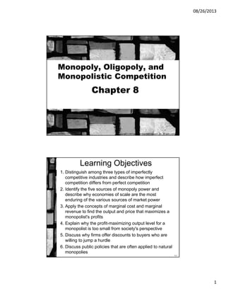
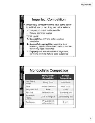
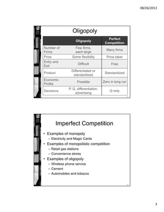
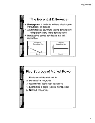
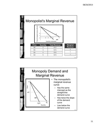
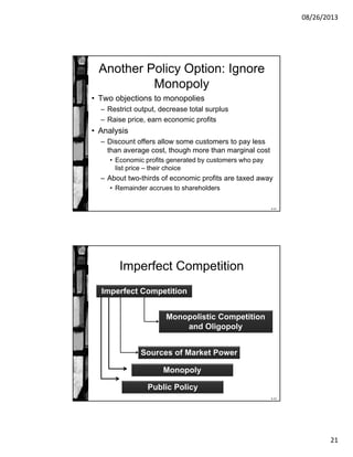
This document provides an overview of imperfect competition, including monopoly, oligopoly, and monopolistic competition. It discusses the key differences between imperfect and perfect competition. Specifically, it covers: 1) The three types of imperfect competition and how they differ from perfect competition in terms of number of firms, price flexibility, entry/exit, and potential for economic profits. 2) The five sources of monopoly power, with a focus on economies of scale as the most enduring source due to decreasing average costs. 3) How monopolists determine profit-maximizing output by setting marginal revenue equal to marginal cost, which results in a smaller output and higher price than the socially optimal level. 4) Examples are provided

1. 08/26/2013
1
Monopoly, Oligopoly, and
Monopolistic Competition
Chapter 8
Copyright © 2013 by The McGraw-Hill Companies, Inc. All rights reserved.McGraw-Hill/Irwin
8-2
Learning Objectives
1. Distinguish among three types of imperfectly
competitive industries and describe how imperfect
competition differs from perfect competition
2. Identify the five sources of monopoly power and
describe why economies of scale are the most
enduring of the various sources of market power
3. Apply the concepts of marginal cost and marginal
revenue to find the output and price that maximizes a
monopolist's profits
4. Explain why the profit-maximizing output level for a
monopolist is too small from society's perspective
5. Discuss why firms offer discounts to buyers who are
willing to jump a hurdle
6. Discuss public policies that are often applied to natural
monopolies

2. 08/26/2013
2
8-3
Imperfect Competition
• Imperfectly competitive firms have some ability
to set their own price: they are price setters
– Long-run economic profits possible
– Reduce economic surplus
• Three types:
1. Monopoly has only one seller, no close
substitutes
2. Monopolistic competition has many firms
producing slightly differentiated products that are
reasonably close substitutes
3. Oligopoly has a small number of large firms
producing products that are close substitutes
8-4
Monopolistic Competition
Monopolistic
Competition
Number of
Firms
Many firms
Price Limited flexibility
Entry and Exit Free
Product Differentiated
Economic
Profits
Zero in long run
Decisions
P, Q, product
differentiation
Perfect
Competition
Many firms
Price taker
Free
Standardized
Zero in long run
Q only

3. 08/26/2013
3
8-5
Oligopoly
Oligopoly
Number of
Firms
Few firms,
each large
Price Some flexibility
Entry and
Exit
Difficult
Product
Differentiated or
standardized
Economic
Profits
Possible
Decisions
P, Q, differentiation,
advertising
Perfect
Competition
Many firms
Price taker
Free
Standardized
Zero in long run
Q only
8-6
Imperfect Competition
• Examples of monopoly
– Electricity and Magic Cards
• Examples of monopolistic competition
– Retail gas stations
– Convenience stores
• Examples of oligopoly
– Wireless phone service
– Cement
– Automobiles and tobacco

4. 08/26/2013
4
8-7
The Essential Difference
• Market power is the firm's ability to raise its price
without losing all its sales
• Any firm facing a downward sloping demand curve
– Firm picks P and Q on the demand curve
• Market power comes from factors that limit
competition
Quantity
Price
Imperfectly
Competitive Firm
D
Quantity
Price
Perfectly
Competitive Firm
D
8-8
Five Sources of Market Power
1. Exclusive control over inputs
2. Patents and copyrights
3. Government licenses or franchises
4. Economies of scale (natural monopolies)
5. Network economies

5. 08/26/2013
5
8-9
Market Power: Economies of
Scale
• Returns to scale refers to the percentage
change in output from a given percentage
change in ALL inputs
– Long-run idea
– Constant returns to scale: doubling all inputs
doubles output
– Increasing returns to scale: output increases by
a greater percentage than the increase in inputs
• Average costs decrease as output increases
• Natural monopoly: a monopoly that results from
economies of scale
8-10
Market Power: Network
Economies
• Network economies occur when the value of
the product increases as the number of users
increases
– VHS format for video tapes, Blu-ray for DVDs
– Telephones
– Windows operating system
– eBay
– Facebook and MySpace

6. 08/26/2013
6
8-11
Economies of Scale and Start-
Up Costs
• New products can have a large fixed development
cost
• Variable cost: sum of payments made to the variable
factors, such as labor
• Fixed cost: sum of payments made to the fixed
factors, such as capital
• Start-up costs can be thought of as a fixed cost
• Average total cost (ATC): total cost divided by output
• A good whose production has a large start-up cost and
low variable cost is subject to economies of scale
– ATC declines sharply as output increases
8-12
Economies of Scale and Start-
Up Costs
• Consider an example:
• Assume marginal cost (M) is constant
• Variable cost is M*Q
• Total cost is fixed cost (F) plus variable cost
TC = F + M*Q
– Total cost increases as output increases
• Average total cost is
ATC = F / Q + M
– Average total cost decreases as output increases
– Average fixed cost = F/Q

7. 08/26/2013
7
8-13
Economies of Scale
Quantity
Totalcost($/year)
F
TC = F + M Q
Averagecost($/unit)
Quantity
ATC = F/Q + M
M
8-14
Example: Video Game
Producers – Different Volumes
Nintendo Playstation
Annual Production
(000s)
1,000 1,200
Fixed Cost ($000s) $200 $200
Variable Cost
($000s)
$800 $960
Total Cost ($000s) $1,000 $1,160
ATC per game $1.00 $0.97

8. 08/26/2013
8
8-15
Example: Video Game Producers
– Lower Marginal Costs
Nintendo Playstation
Annual Production
(000s)
1,000 1,200
Fixed Cost ($000s) $200 $200
Variable Cost
($000s)
$200 $240
Total Cost ($000s) $400 $440
ATC per game $0.40 $0.37
8-16
Example: Video Game
Producers – Higher Fixed Cost
Nintendo Playstation
Annual Production
(000s)
1,000 1,200
Fixed Cost ($000s) $10,000 $10,000
Variable Cost
($000s)
$200 $240
Total Cost ($000s) $10,200 $10,240
ATC per game $10.20 $8.53

9. 08/26/2013
9
8-17
Example: Video Game Producers –
Different Production Levels
Nintendo Playstation
Annual Production
(000s)
500 1,700
Fixed Cost ($000s) $10,000 $10,000
Variable Cost
($000s)
$100 $340
Total Cost ($000s) $10,100 $10,240
ATC per game $20.20 $6.08
8-18
Intel's Advantage
• Development cost of a new chip $2 billion
• Marginal cost of making a chip Pennies
• Dominating the market Priceless
• Intel supplies more than 80% of the processors
for PCs

10. 08/26/2013
10
8-19
Profit Maximization for the
Monopolist
• Like all other firms, a monopolist:
– Maximizes profits
– Applies the Cost-Benefit Principle:
• Increase output if marginal benefit > marginal cost
• Decrease output is marginal benefit < marginal cost
• Marginal benefit is called marginal revenue:
– Change in total revenue from a one-unit change in
output
– Equal to price for the perfectly competitive firm
– Less than price for the monopolist
8-20
Price($/unit)
Quantity (units/week)
Profit Maximization for the
Monopolist
• To sell another unit the monopolist must lower price
– Total revenue from 2 units = $12
– Total revenue from 3 units = $15
• Marginal revenue = $3
D
2
6
3
5

11. 08/26/2013
11
8-21
Monopolist's Marginal Revenue
Total Revenue
$12
$15
$16
$15
Price Quantity
$6 2
$5 3
$4 4
$3 5
Price&marginalrevenue($/unit) 8
8
D
Quantity (units/week)
MR
32
3
1
4-1 5
Marginal
Revenue
3
1
-1
8-22
Monopoly Demand and
Marginal Revenue
• The monopolist's
marginal revenue
curve:
– Has the same
intercept as the
straight-line
demand curve
– Has twice the slope
of the demand
curve
– Lies below the
demand curve
Price
Quantity
a
D
Q0
Q0/2
a/2
MR

12. 08/26/2013
12
8-23
Deciding Quantity
• Profit is maximized at the
level of output where
marginal cost equals
marginal revenue
• At P = $3 and Q = 12,
MC > MR
• Decrease output
– At Q = 8, MC = MR = 2
• The demand curve sets the
price at P = $4
– At any output below 8,
MC < MR
Price($/unitofoutput) Quantity (units/week)
3
MC
2
6
D
12
MR
4
8
8-24
Monopoly Profit
• Profit = Total revenue – total cost
• Total cost = ATC x Q
• Profit = P x Q – ATC x Q
• Profit = (P-ATC) x Q
• If P > ATC then the firm earns a profit
• If P < ATC then the firm suffers a loss
• This can be graphically illustrated

13. 08/26/2013
13
8-25
Monopoly Losses and Profits
Price($/minute)
Minutes (millions/day)
20
0.12
0.10
ATC
Economic loss
= $400,000/day
D
0.05 MC
MR
24
Price($/minute)
Minutes (millions/day)
2420
0.08
0.10
ATC
D
0.05 MC
MR
Economic profit
= $400,000/day
8-26
The Invisible Hand Fails
Price($/unitofoutput)
Quantity (units/week)
The socially optimal
amount occurs where
MC = MB, Q = 12 units
and P = $3
The monopolist's optimal
amount occurs where
MC = MR, Q = 8 units
and P = $4
2
MR
8
4
24
D
3
12
6 Marginal Cost
Deadweight loss
from monopoly = $4

14. 08/26/2013
14
8-27
Monopoly and Perfect
Competition
Monopoly
MC = MR
P >MR
P > MC
Deadweight
Loss
Perfect Competition
MC = MR
P = MR
P = MC
No Deadweight
Loss
8-28
Managing Monopoly: The
Breakdown of the Invisible Hand
• Monopolies exist for economic reasons
– Patents, copyrights, and innovation
– Economies of scale
– Network economies
• Anti-trust laws attempt to limit deadweight loss
– Limiting monopoly has costs
• Patents encourage innovation
• Economies of scale minimize ATC
• Network economies increase benefits

15. 08/26/2013
15
8-29
Price Discrimination
• Price discrimination means charging different
buyers different prices for essentially the same
good or service
– Separate the groups
– No side trades among buyers
• Many forms of price discrimination
– Hurdle method: discounts for identifiable groups
(e. g., students, AARP)
– Perfect discrimination: negotiate separate deals
with each customer
8-30
Carla the Editor: Social Optimum
• Opportunity cost of Carla's time is $29
What is the
social optimum?
What if Carla
is a profit
maximizer?
What is
Carla's total
revenue?
Student
Reservation
Price
A $40
B 38
C 36
D 34
E 32
F 30
G 28
Total
Revenue
$40
$76
$108
$136
$160
$180
$196
6 papers with
an economic
profit of $6

16. 08/26/2013
16
8-31
Carla the Editor: Marginal Revenue
• Opportunity cost of Carla's time is $29
What is Carla's
marginal revenue?
Student
Reservation
Price
A $40
B 38
C 36
D 34
E 32
F 30
G 28
MR
$40
$36
$32
$28
$24
$20
$16
Total
Revenue
$40
$76
$108
$136
$160
$180
$196
3 papers with an
economic profit of
$21
8-32
Carla the Editor: Price Discriminator
• Opportunity cost of Carla's time is $29
What if Carla is a perfect price
discriminator?
What is Carla's
total revenue?
Student
Reservation
Price
A $40
B 38
C 36
D 34
E 32
F 30
G 28
Total
Revenue
$40
$78
$114
$148
$180
$210
$238
6 papers with
an economic
profit of $36

17. 08/26/2013
17
8-33
Hurdle Method of Price
Discrimination
• The hurdle method of price discrimination is the
practice of offering a discount to all buyers who
overcome some obstacle.
– Temporary sales
– Hard cover and paperback books
– Multiple car models from one manufacturer
– Commercial air carriers
– Movie producers and phased releases
– Scratch and Dent appliance sales
8-34
Carla Offers a Rebate
• If reservation price < $36, student will mail in rebate
Student
Reservation
Price
Total
Revenue
A $40 $40
B 38 76
C 36 108
Discounted Price Submarket
D $34 $34
E 32 64
F 30 90
MR
$40
36
32
$34
30
26
5 papers, price $36, rebate
$4, economic profit $27

18. 08/26/2013
18
8-35
Carla's Choices
Program
Social
Optimum
Papers Edited 6
Price $30
Total Revenue $180
Carla's Time $174
Economic Profit $6
Total Surplus $26
Hurdle
5 = (3 + 2)
$36, $4
rebate
$172
$145
$27
$35
Perfect
Discriminator
6
Reservation
$210
$174
$36
$36
Single
Price
3
$36
$108
$87
$21
$27
8-36
Monopoly and Public Policy
• Challenge: create the greatest increase in total
surplus
• Policy options
– Government ownership and operation
– Regulation
– Competitive bids for natural monopoly services
– Break up

19. 08/26/2013
19
8-37
State-Owned Natural Monopoly
• Marginal cost is always less than average cost
– Marginal cost pricing produces losses
• Options
– Fund losses from tax revenues
– Fixed monthly fee plus usage fee
• Fixed fee covers losses
• Limited incentives to innovate and cut costs
• Commonly used for water, Post Office, and some
electricity
8-38
Regulated Monopolies
• Cost-plus regulation sets price at per unit
explicit costs plus a mark-up for implicit costs
• Used for electricity, telephone, and cable
– Policies vary by state
• Disadvantages
– High administrative cost
– Reduced incentive for cost-saving innovation
– Price is greater than marginal cost

20. 08/26/2013
20
8-39
Exclusive Contracting for
Natural Monopolies
• Government awards contract to low bidder for
natural monopoly services
– Garbage collection, fire protection, road construction,
Department of Defense
• Could achieve marginal cost pricing IF
government pays the resulting losses
• Asset transfer for large fixed investment is
complex
8-40
Enforcement of Anti-Trust Laws
• Two landmark laws
– Sherman Act of 1890
• Declared conspiracy to create a monopoly illegal
– Clayton Act of 1914
• Outlawed transactions that would "substantially lessen
competition"
• Applies to mergers and acquisitions today
– IBM avoided break-up; AT&T did not
– Microsoft survived

21. 08/26/2013
21
8-41
Another Policy Option: Ignore
Monopoly
• Two objections to monopolies
– Restrict output, decrease total surplus
– Raise price, earn economic profits
• Analysis
– Discount offers allow some customers to pay less
than average cost, though more than marginal cost
• Economic profits generated by customers who pay
list price – their choice
– About two-thirds of economic profits are taxed away
• Remainder accrues to shareholders
8-42
Imperfect Competition
Imperfect Competition
Monopolistic Competition
and Oligopoly
Sources of Market Power
Monopoly
Public Policy

22. 08/26/2013
22
Chapter 8 Appendix
The Algebra of
Monopoly
Maximization
8-44
From Demand to Marginal
Revenue
• Given a demand curve such as
P = 15 – 2 Q
• We can write the marginal revenue curve as
MR = 15 – 4 Q
• Suppose marginal cost is a line with zero intercept
and a slope of 1
MC = Q
• The remaining step is to set marginal revenue
equal to marginal cost

23. 08/26/2013
23
8-45
MR = MC
• Let Q* be the profit maximizing level of output
MC = MR
Q* = 15 – 4 Q*
5 Q* = 15
Q* = 3
• To find P, substitute Q = 3 into the demand
equation
P = 15 – 4 Q*
P = 15 – 4 (3)
P = 3