Download as PDF, PPTX


![Orientation Assignment
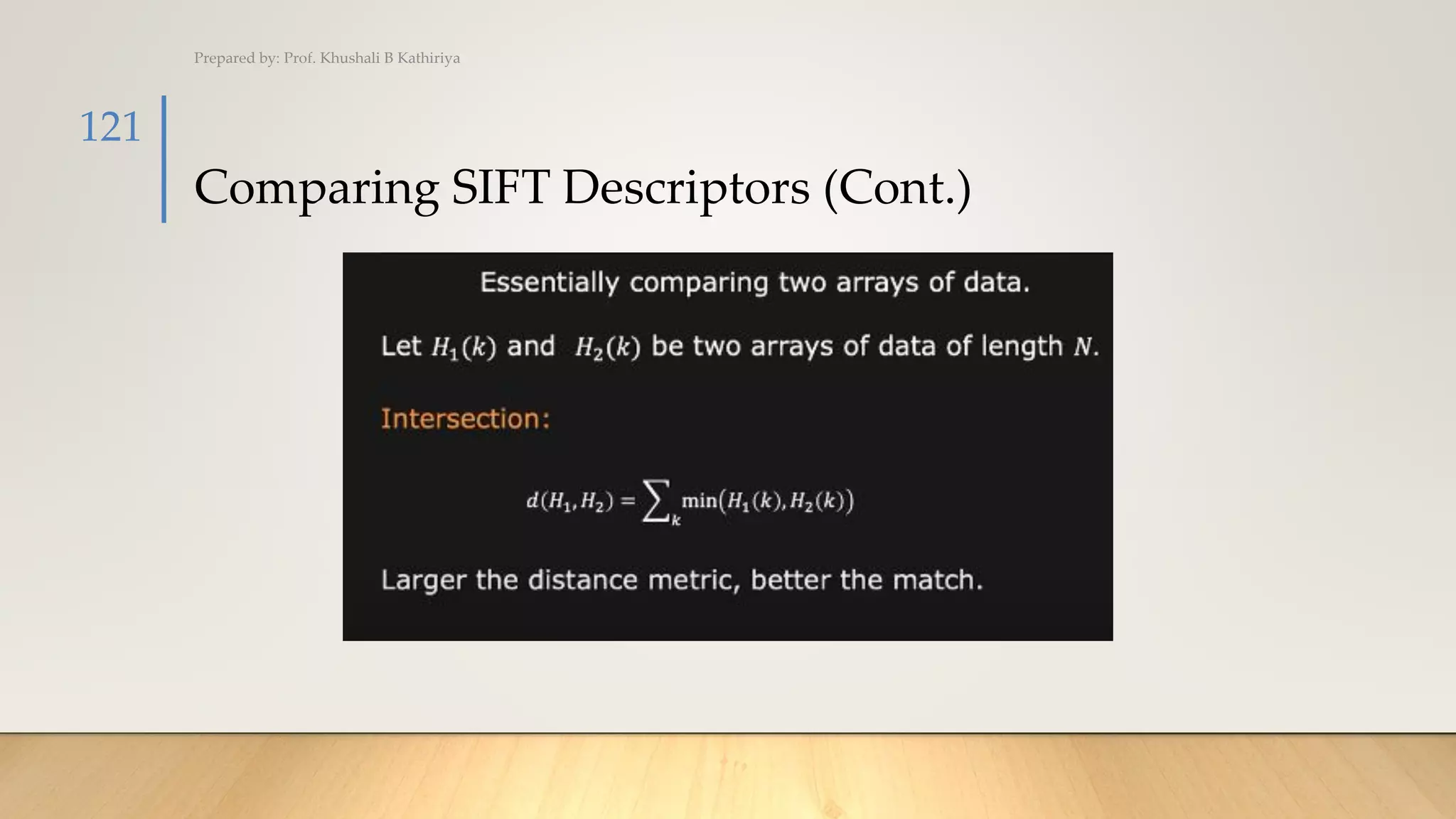
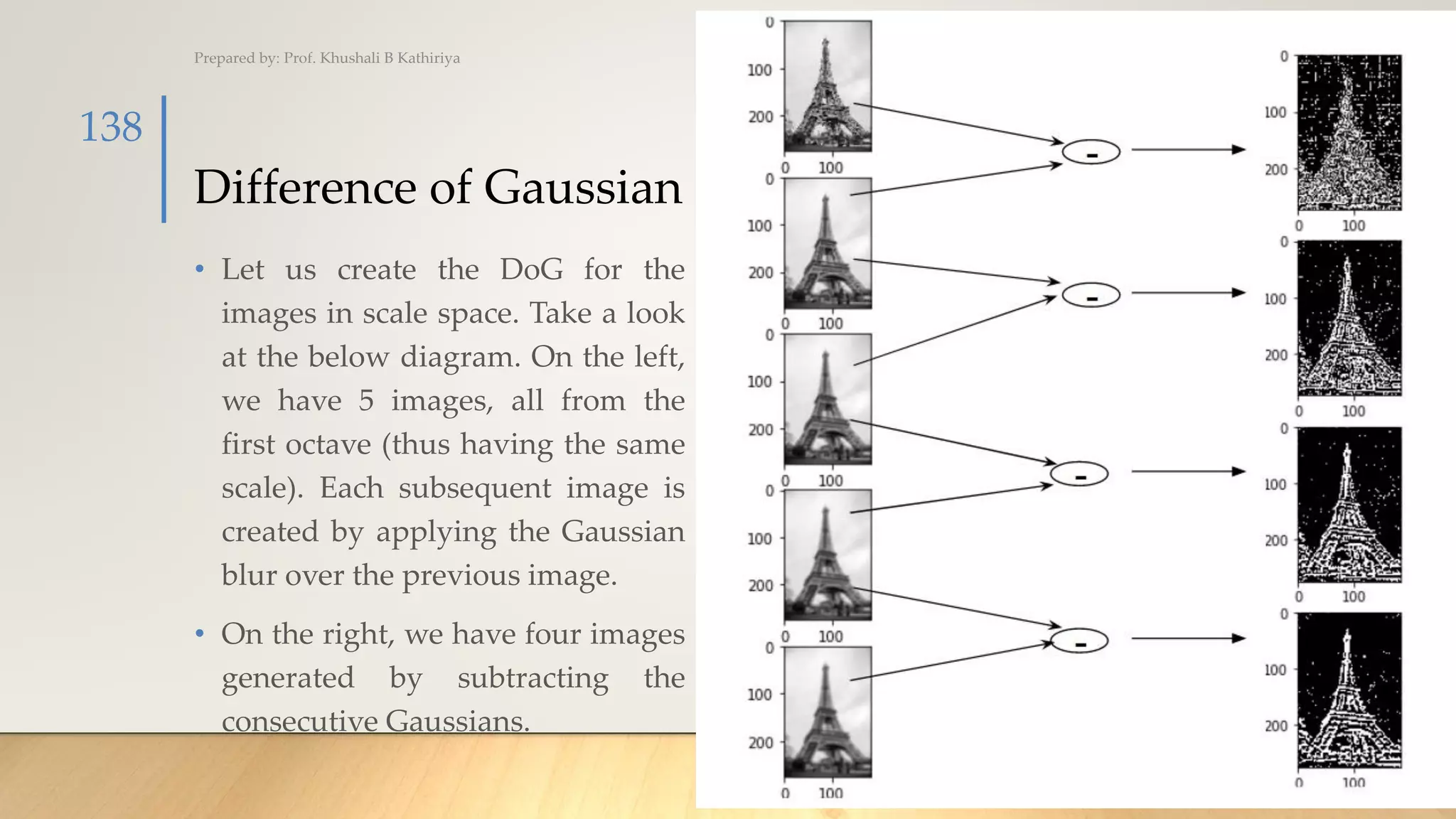
• Let’s say we want to find the magnitude and orientation for
the pixel value in red. For this, we will calculate the
gradients in x and y directions by taking the difference
between 55 & 46 and 56 & 42. This comes out to be Gx = 9
and Gy = 14 respectively.
• Once we have the gradients, we can find the magnitude and
orientation using the following formulas:
• Magnitude = √[(Gx)2+(Gy)2] = 16.64
• Φ = atan(Gy / Gx) = atan(1.55) = 57.17
Prepared by: Prof. Khushali B Kathiriya
142](https://image.slidesharecdn.com/chap3-220124122943/75/CV_Chap-3-Features-Detection-142-2048.jpg)


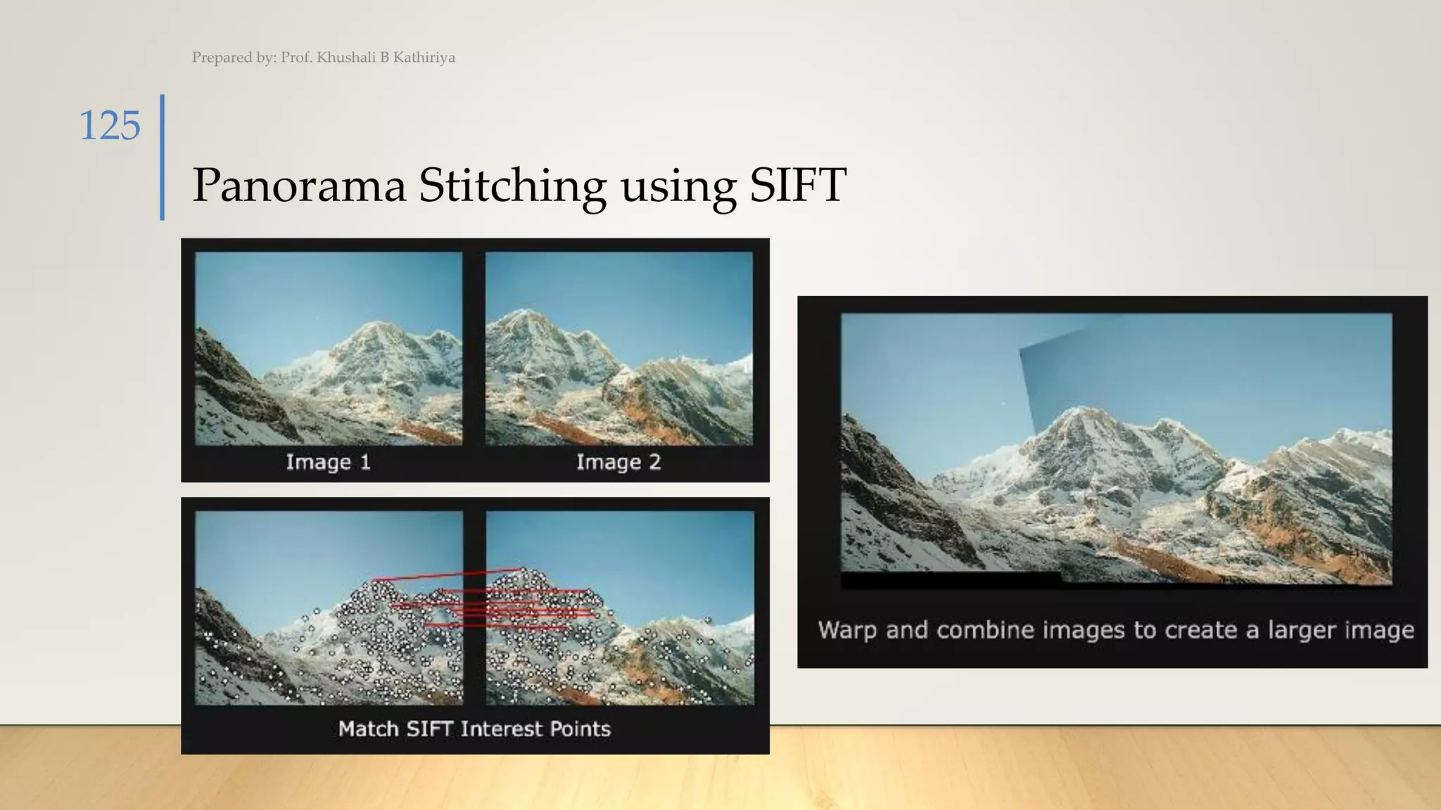
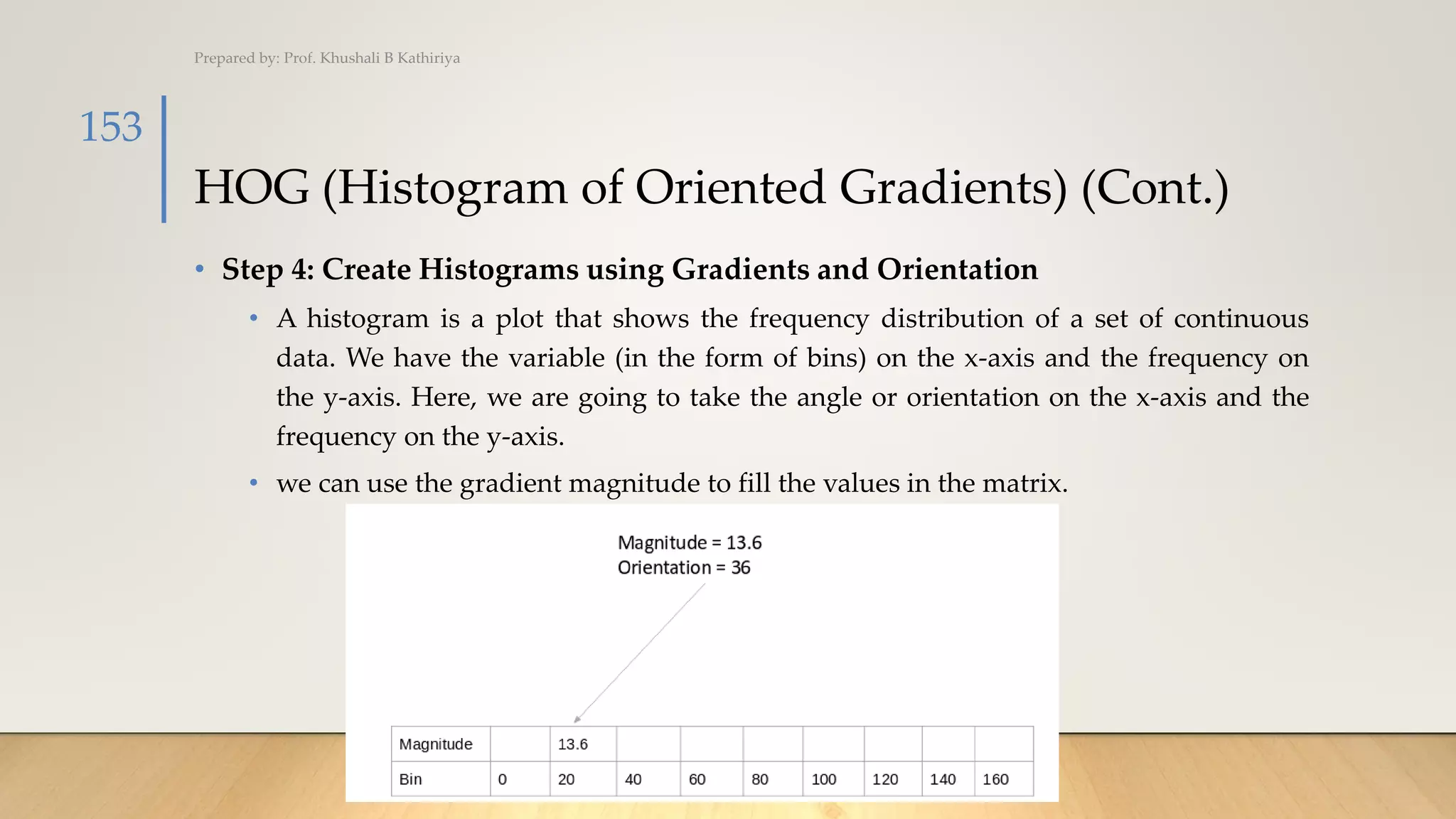
![HOG (Histogram of Oriented Gradients) (Cont.)
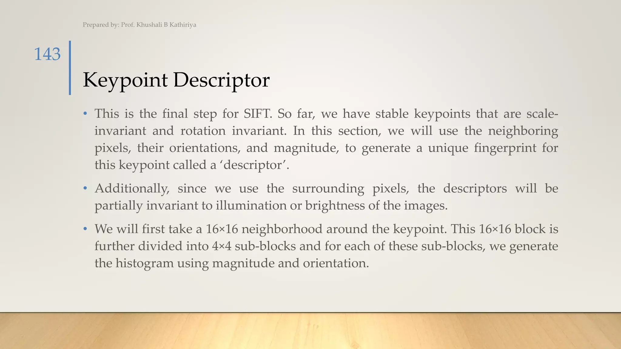
• Step 3: Calculate the Magnitude and Orientation
• The gradients are basically the base and perpendicular here. So, for the previous
example, we had Gx and Gy as 11 and 8. Let’s apply the Pythagoras theorem to
calculate the total gradient magnitude:
• Total Gradient Magnitude = √[(Gx)2+(Gy)2]
• Total Gradient Magnitude = √[(11)2+(8)2] = 13.6
• Next, calculate the orientation (or direction) for the same pixel. We know that we can
write the tan for the angles:
• tan(Φ) = Gy / Gx
• Hence, the value of the angle would be:
• Φ = atan(Gy / Gx) =atan(8/11)= 36
Prepared by: Prof. Khushali B Kathiriya
152](https://image.slidesharecdn.com/chap3-220124122943/75/CV_Chap-3-Features-Detection-152-2048.jpg)
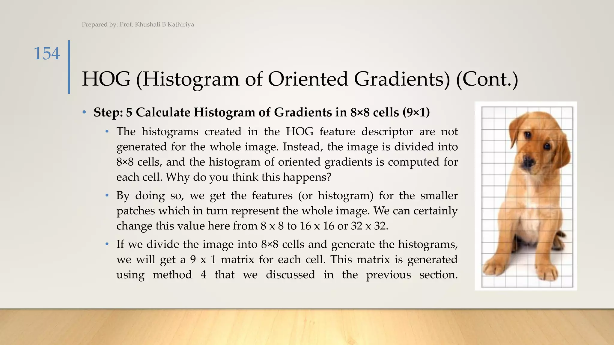


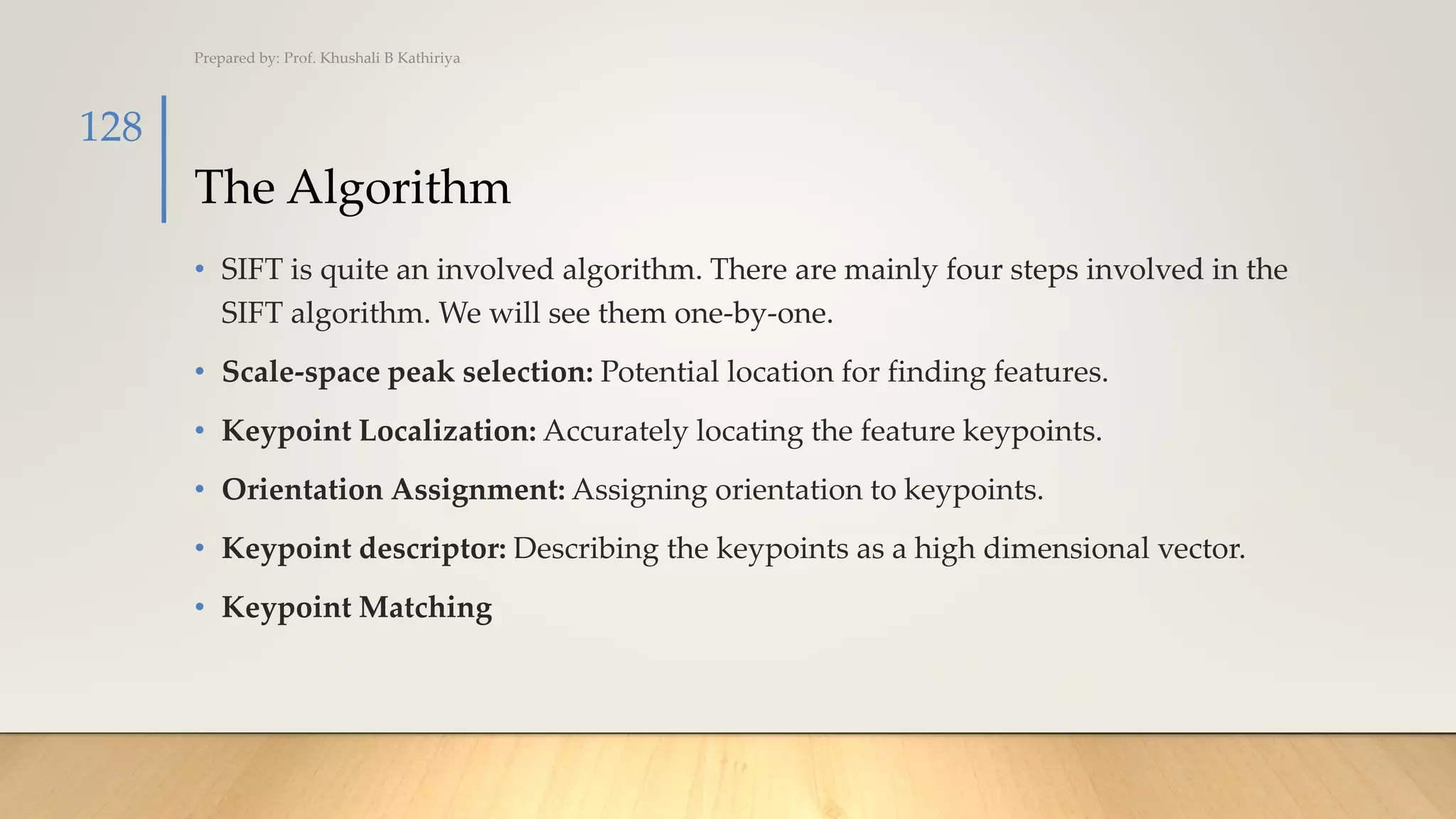
![HOG (Histogram of Oriented Gradients) (Cont.)
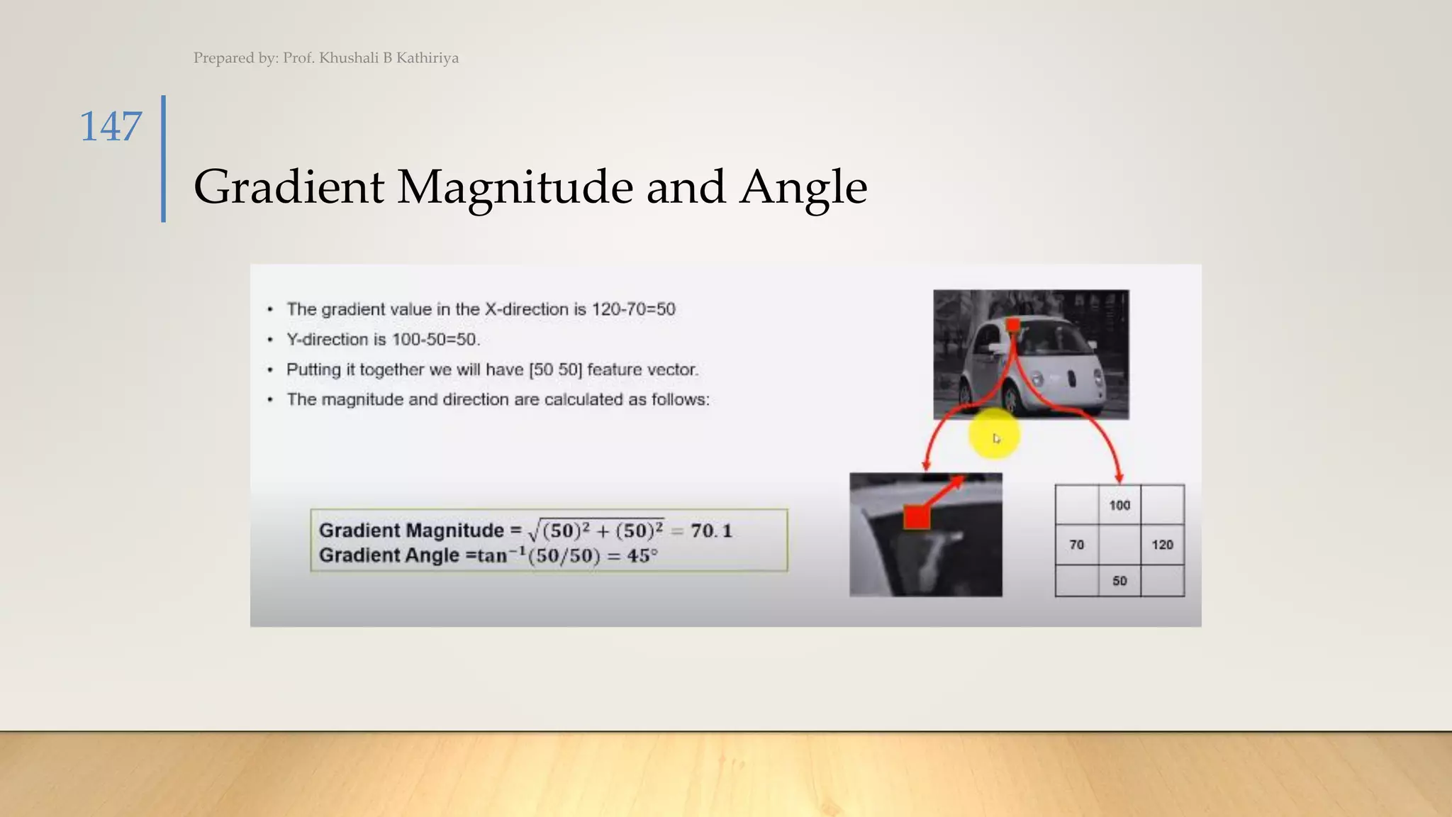
• Here, we will be combining four 8×8 cells to create a 16×16 block. And we already
know that each 8×8 cell has a 9×1 matrix for a histogram. So, we would have four 9×1
matrices or a single 36×1 matrix. To normalize this matrix, we will divide each of
these values by the square root of the sum of squares of the values. Mathematically,
for a given vector V:
• V = [a1, a2, a3, ….a36]
• We calculate the root of the sum of squares:
• k = √(a1)2+ (a2)2+ (a3)2+ …. (a36)2
• And divide all the values in the vector V with this value k:
Prepared by: Prof. Khushali B Kathiriya
157](https://image.slidesharecdn.com/chap3-220124122943/75/CV_Chap-3-Features-Detection-157-2048.jpg)


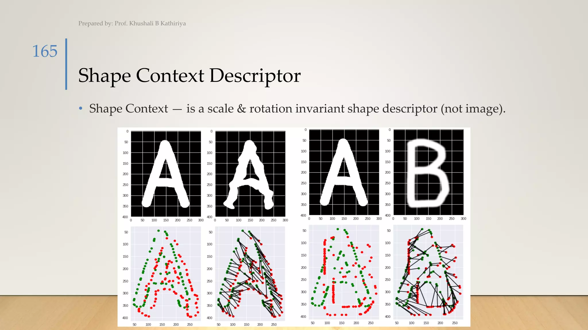


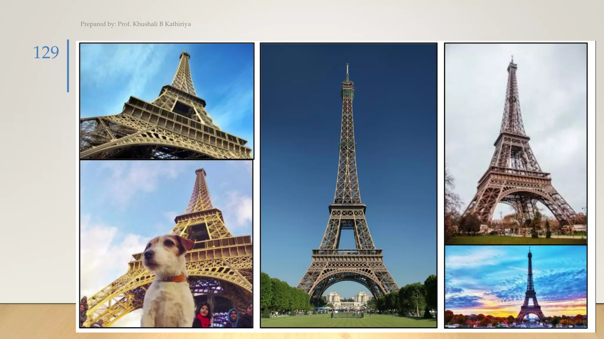
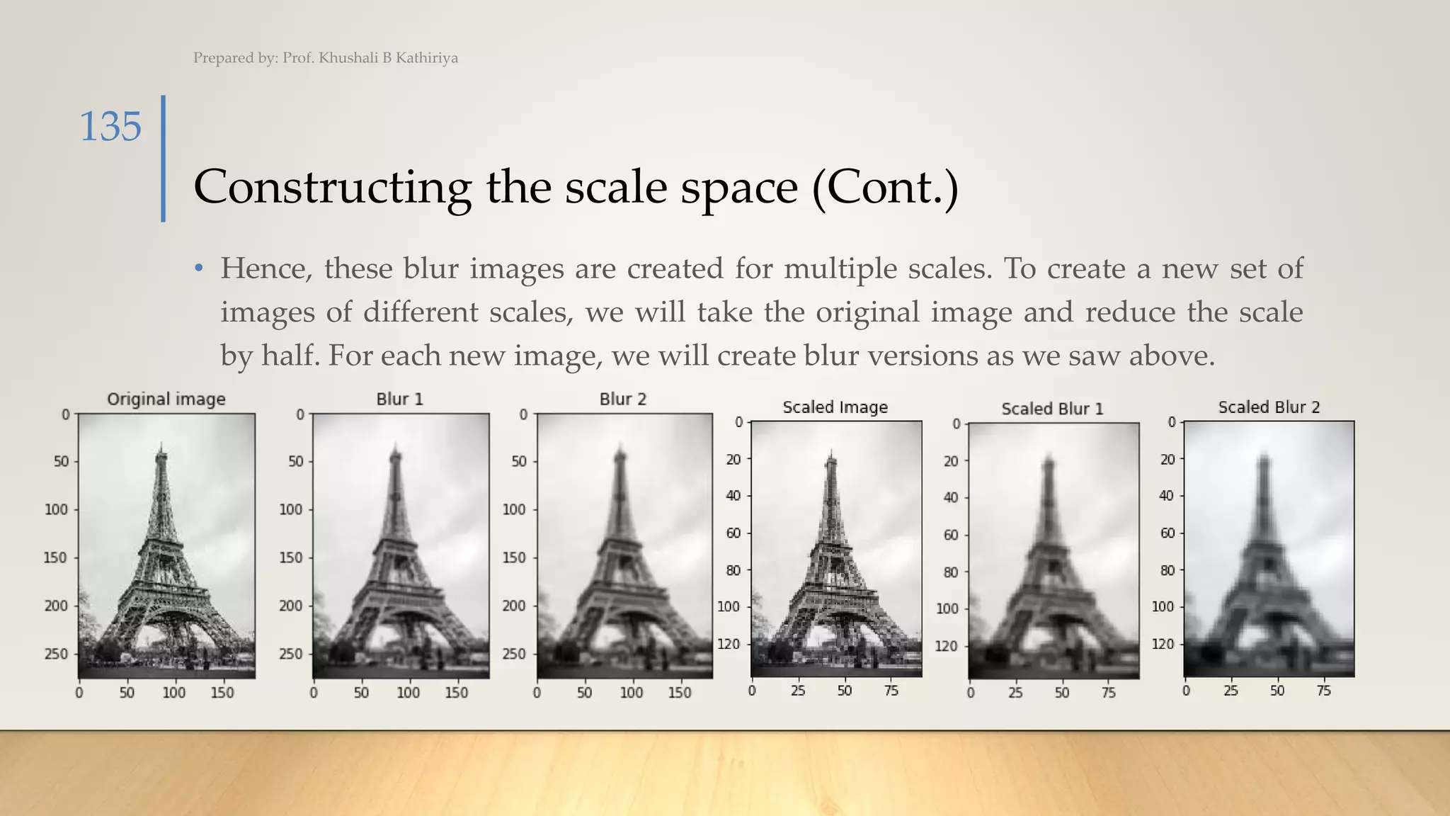
![Shape Context Descriptor (Cont.)
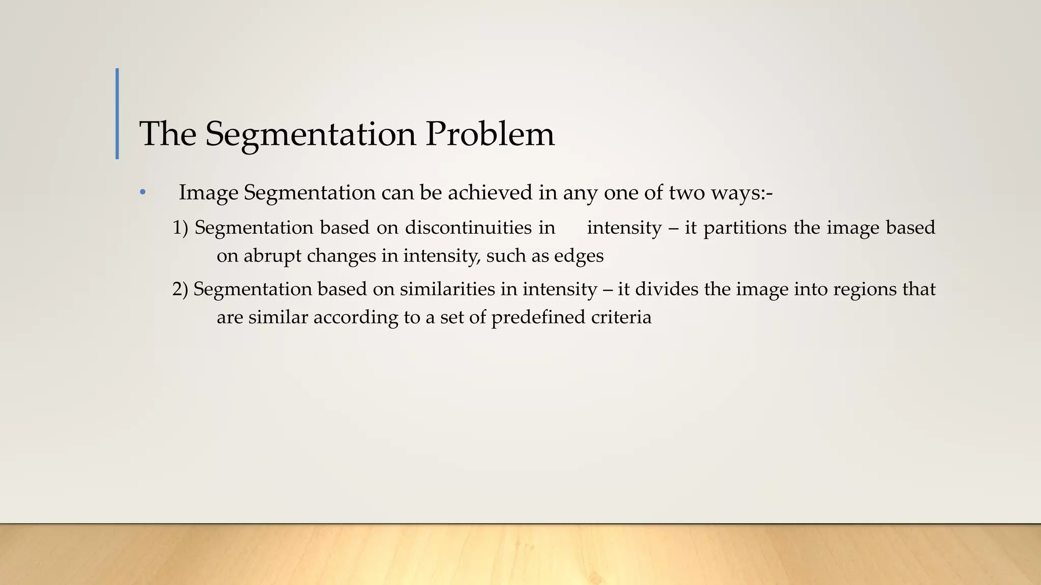
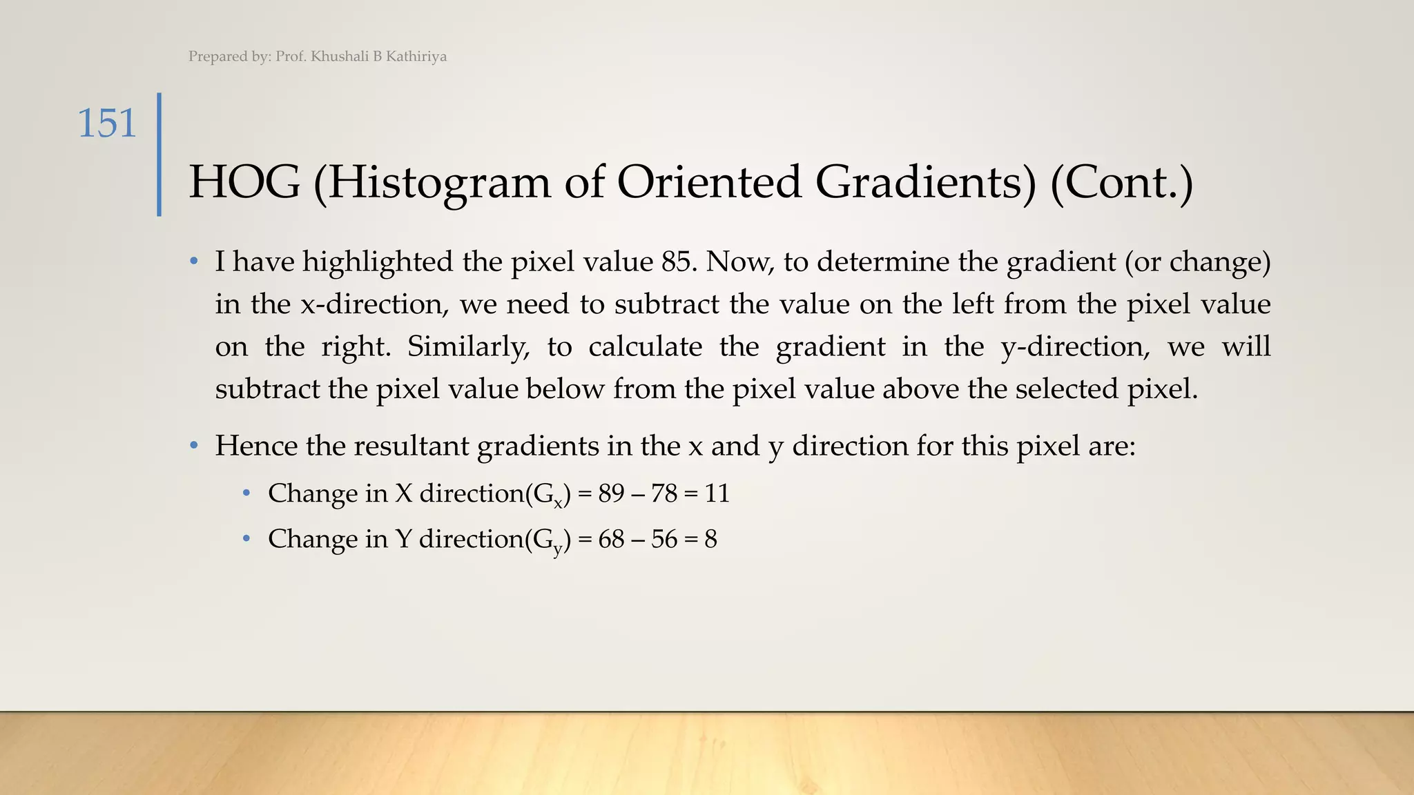
• A logical grid of constant size is applied on boundary image, and we extract
points which are intersecting logical grid with boundary image as shown in
Figure 10. The set of such descriptor points is used for computing feature
descriptor representing shape information of an image.
• The relative arrangement of this descriptor points is represented using the log-
polar histogram. For each descriptor point, the log-polar histogram is calculated,
and last feature descriptor represents the summation of every log-polar
histogram at every descriptor points [7].
Prepared by: Prof. Khushali B Kathiriya
170](https://image.slidesharecdn.com/chap3-220124122943/75/CV_Chap-3-Features-Detection-170-2048.jpg)

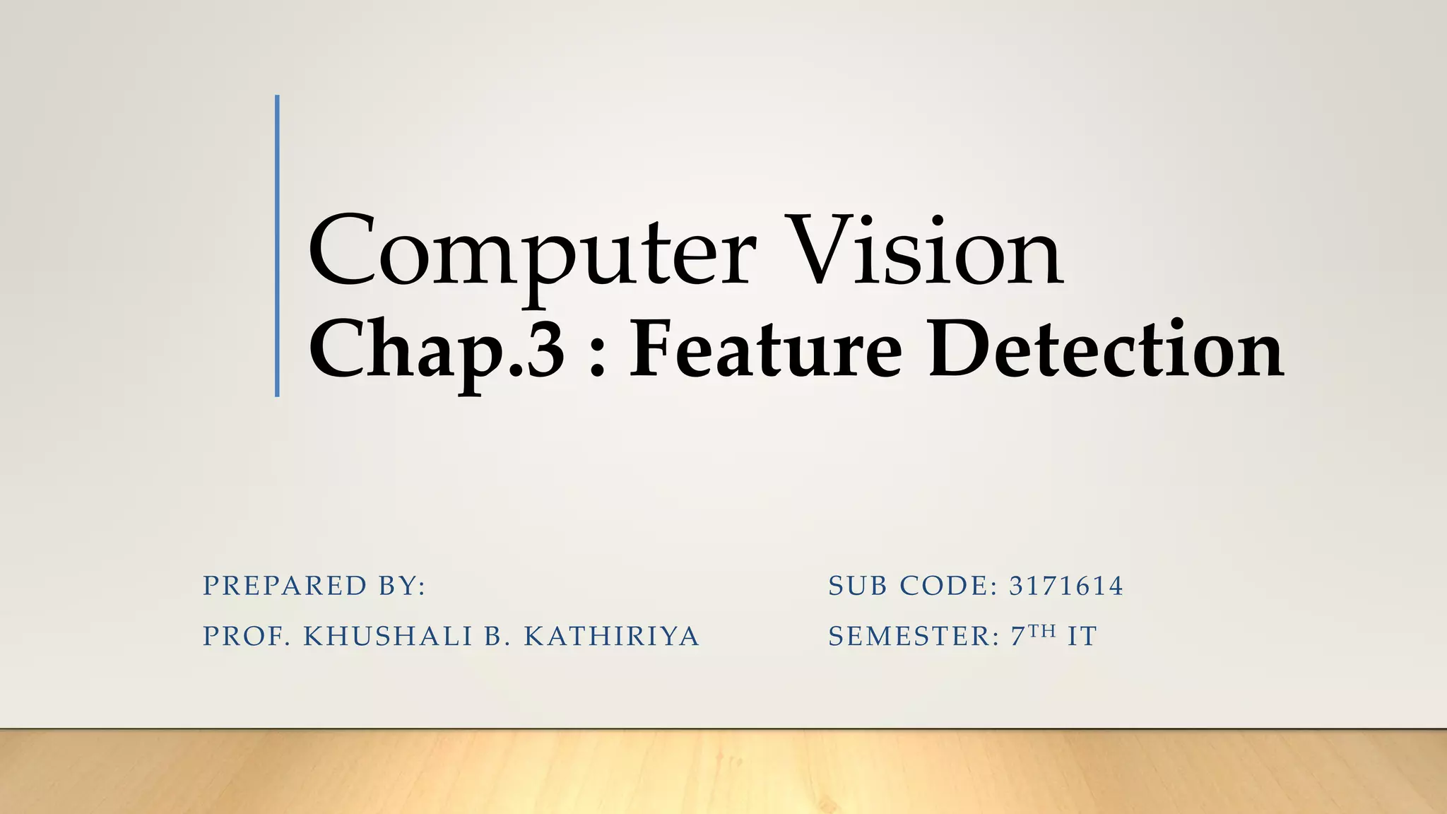
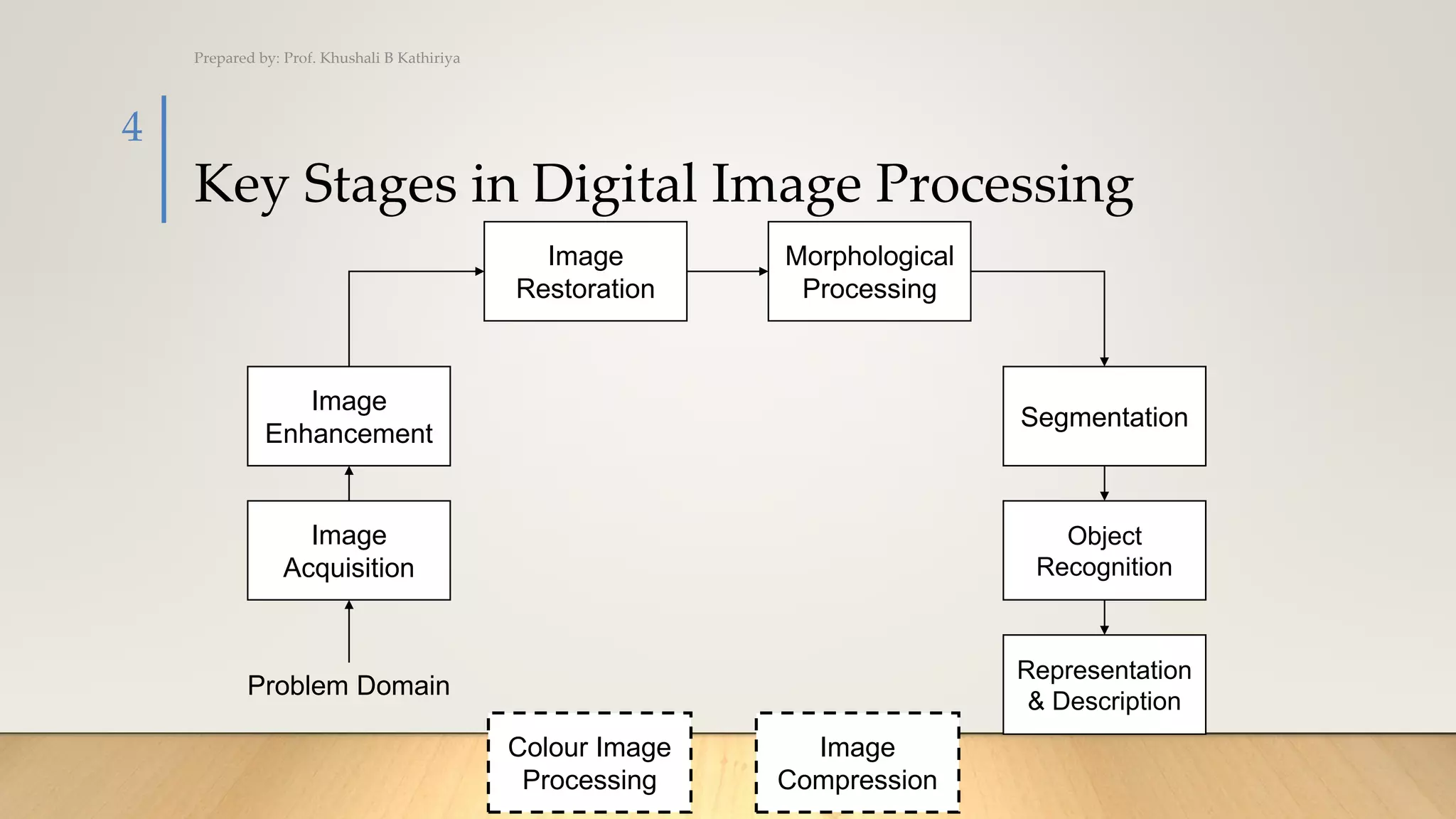
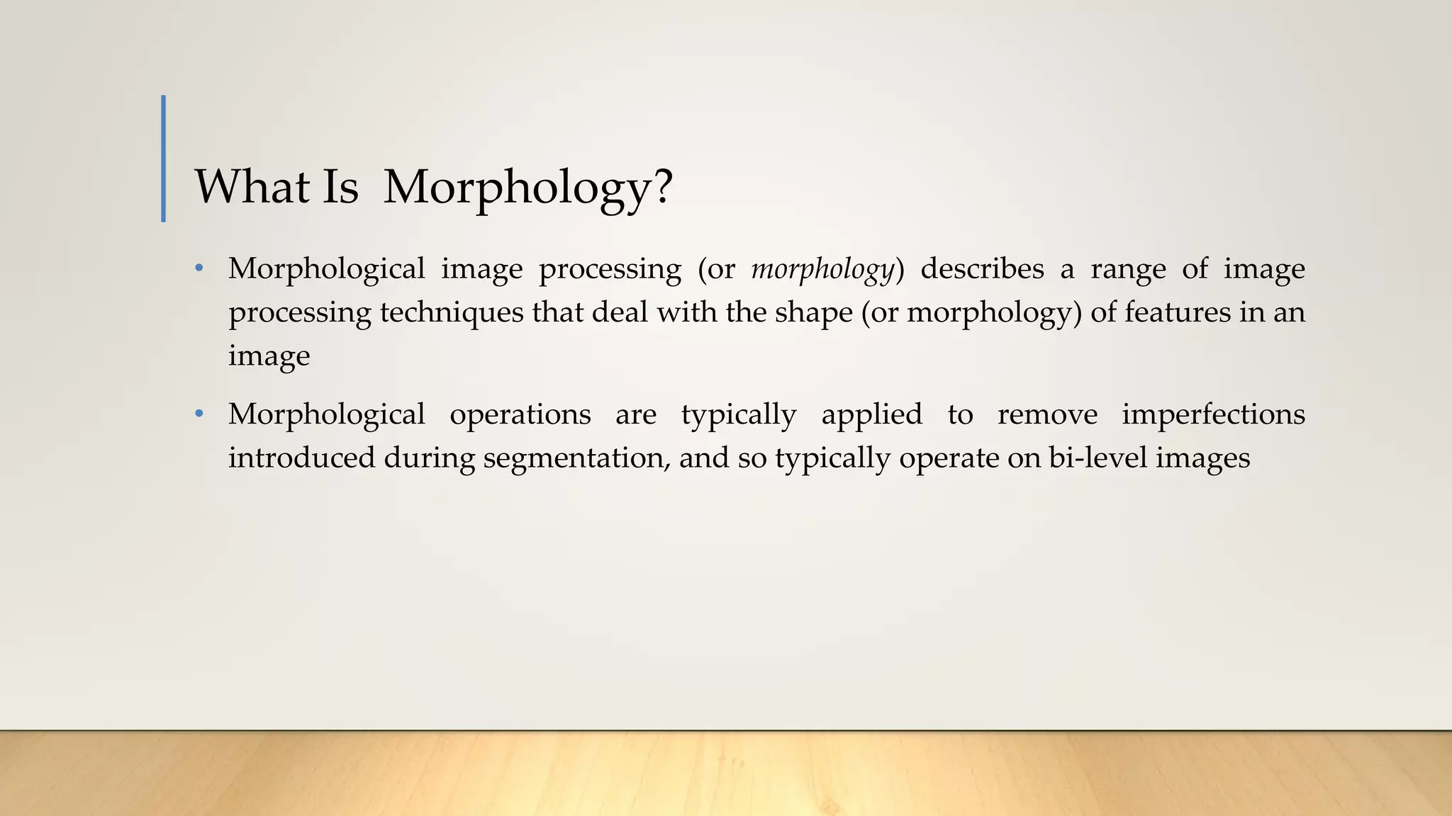
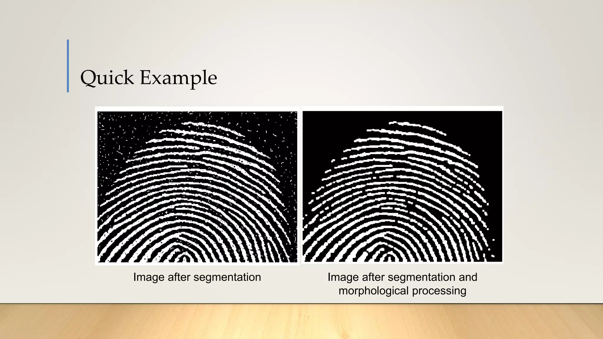
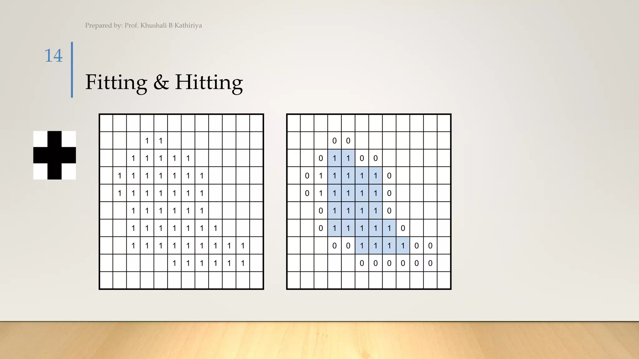
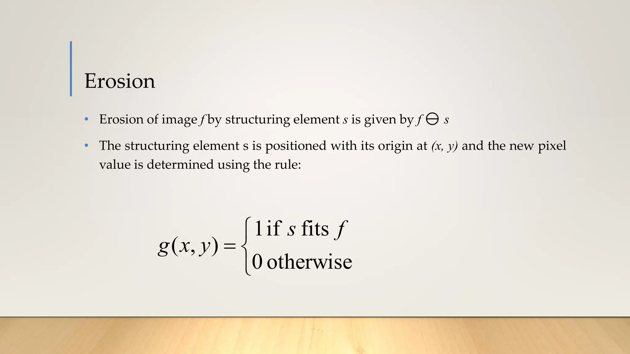
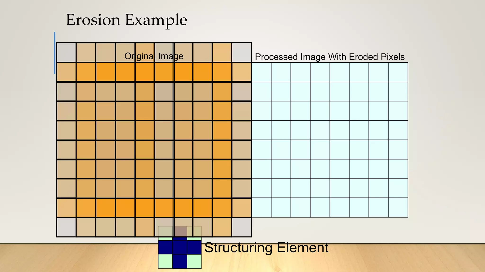
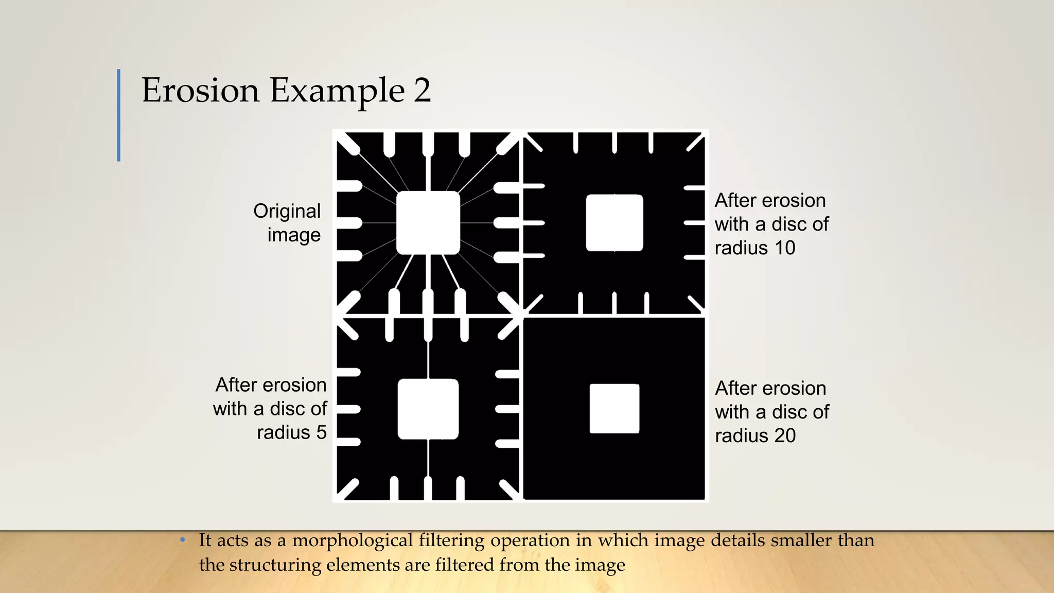
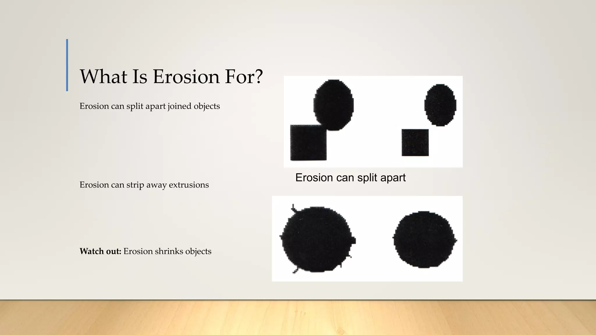
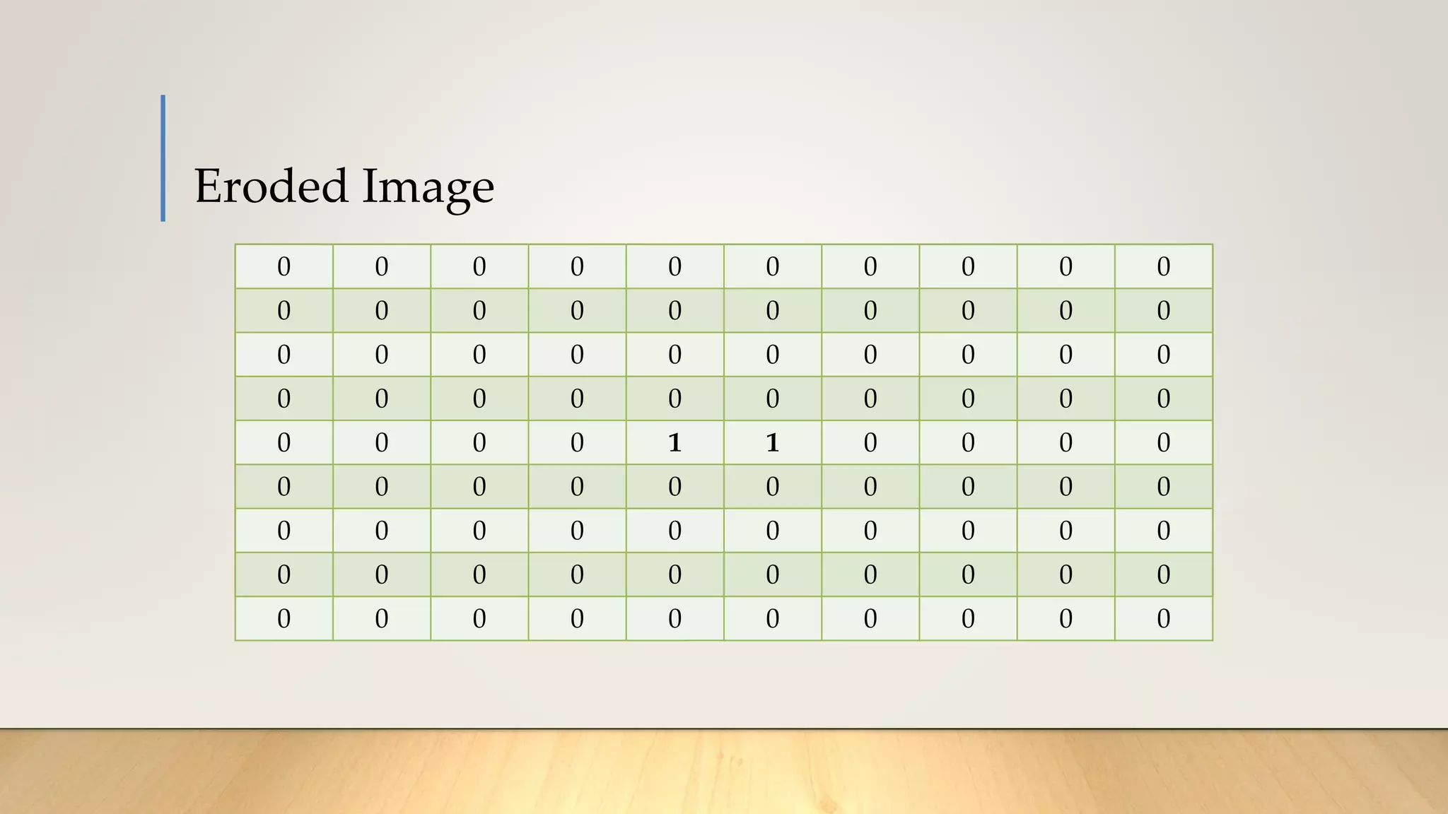
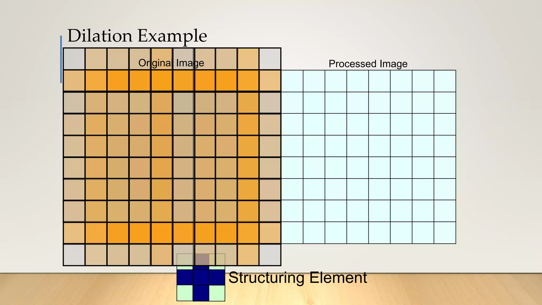
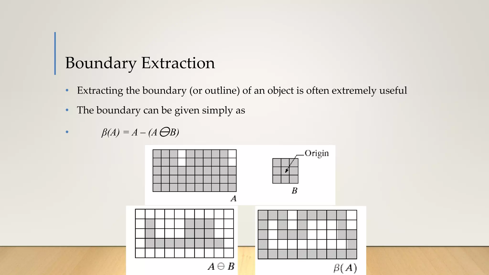
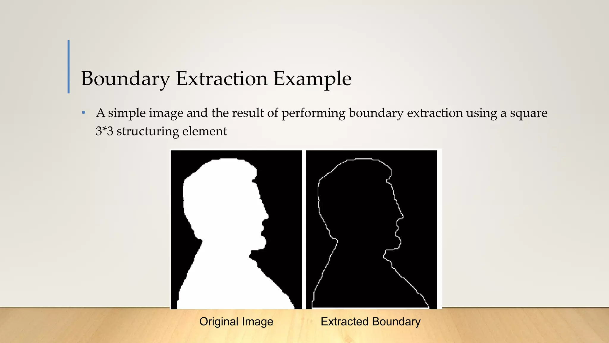
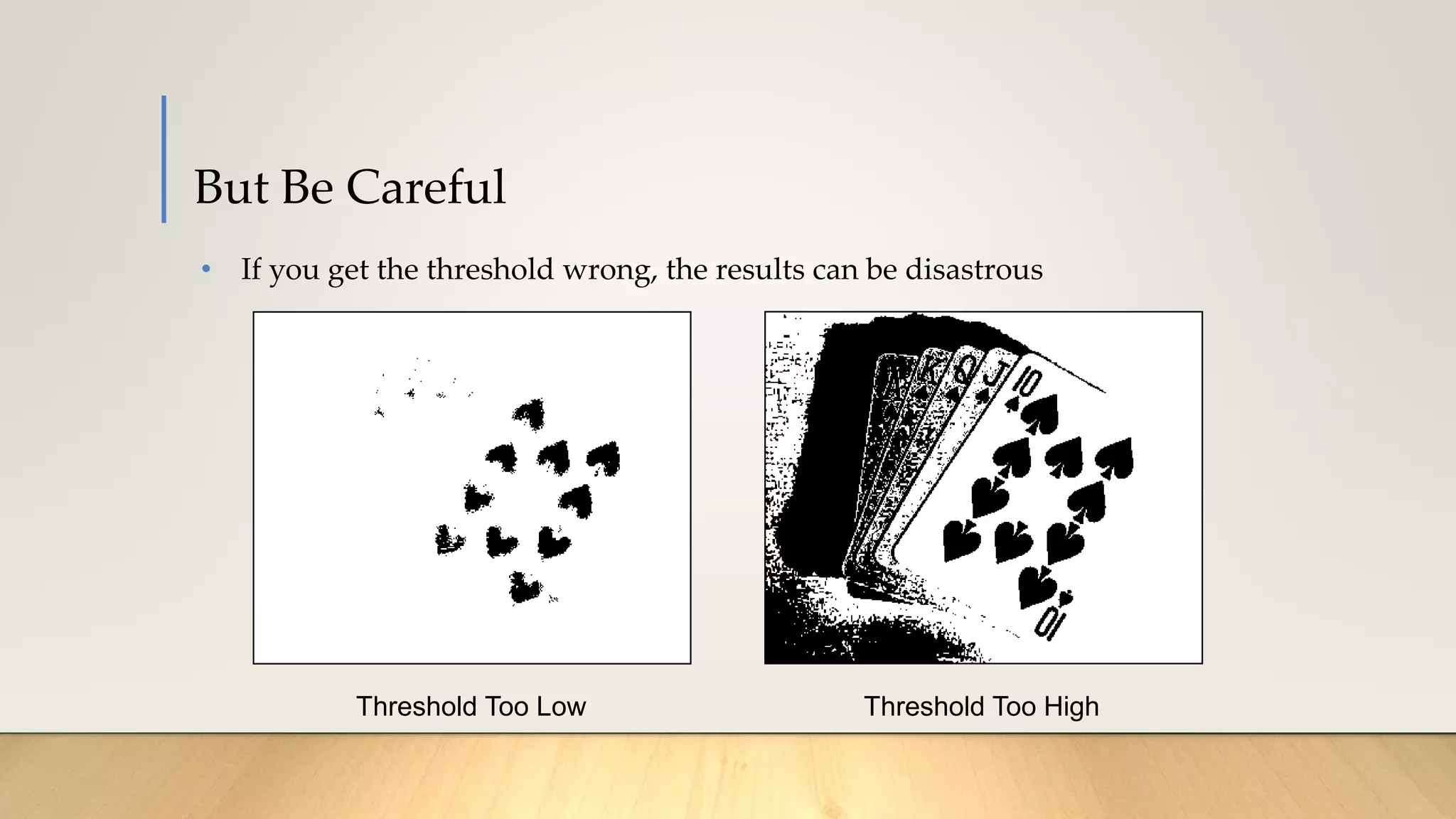
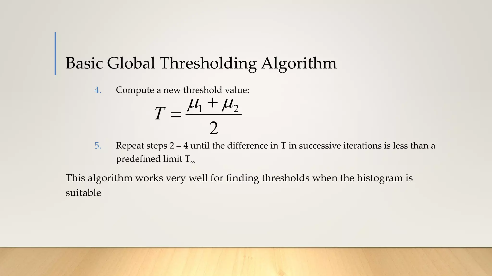
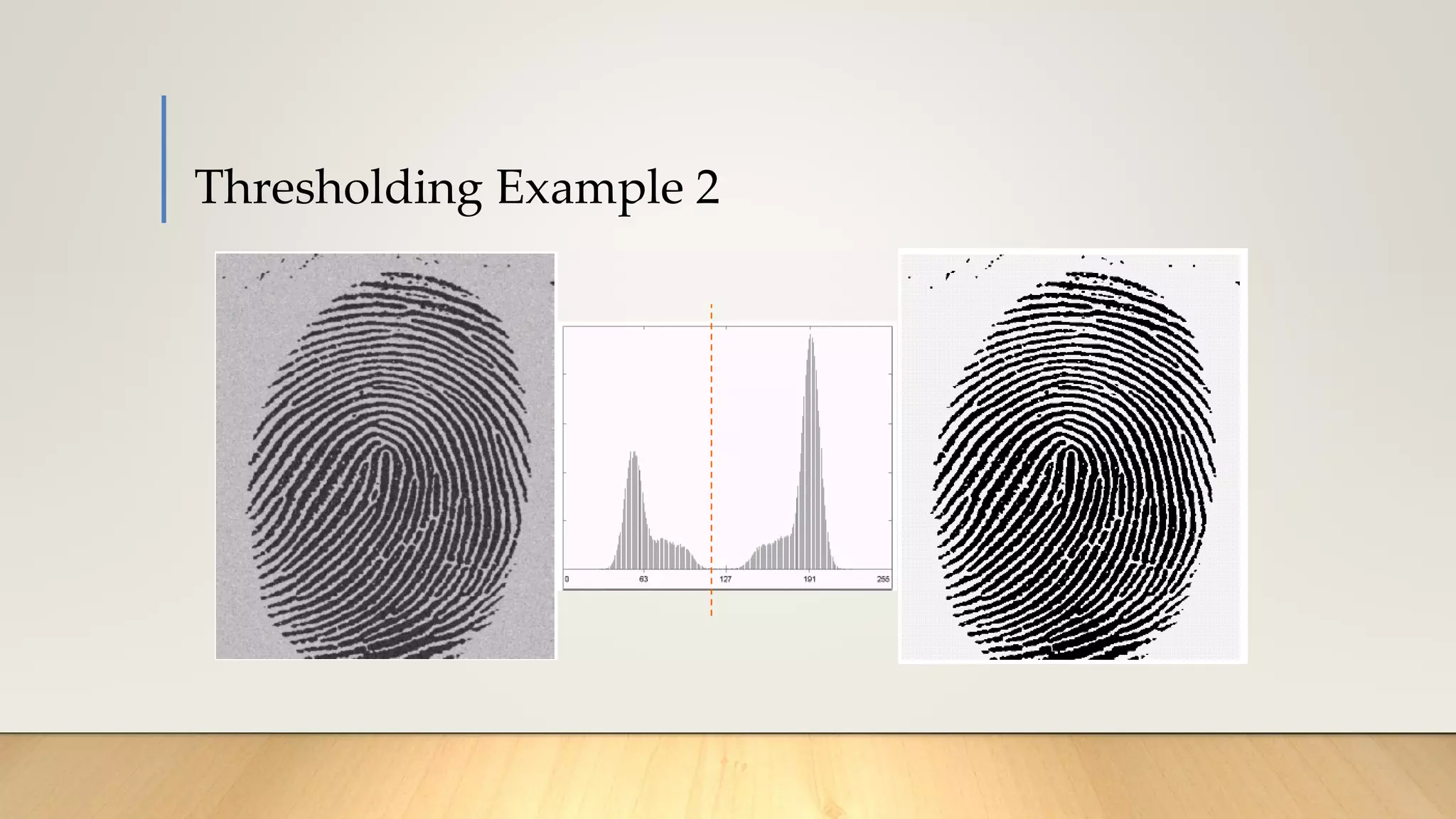
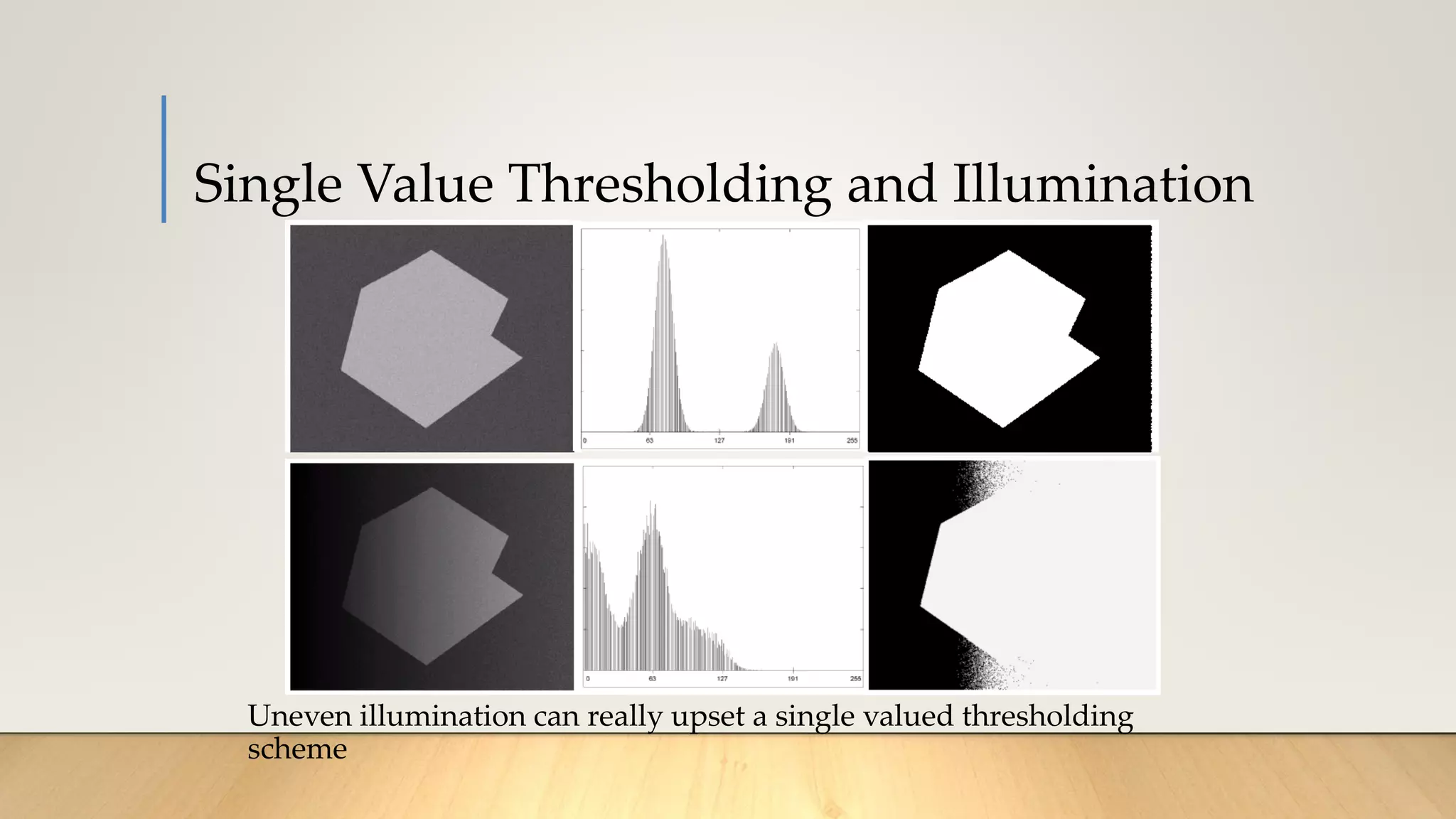
This document discusses various techniques in computer vision, particularly focusing on morphological image processing, which includes operations like erosion and dilation that deal with the shape of features within an image. It outlines key stages in digital image processing such as image acquisition, restoration, and segmentation, and explains how morphological operations can enhance or modify segmented images. Additionally, the document covers thresholding methods for image segmentation, highlighting the differences between global and adaptive thresholding and addressing common challenges during the segmentation process.