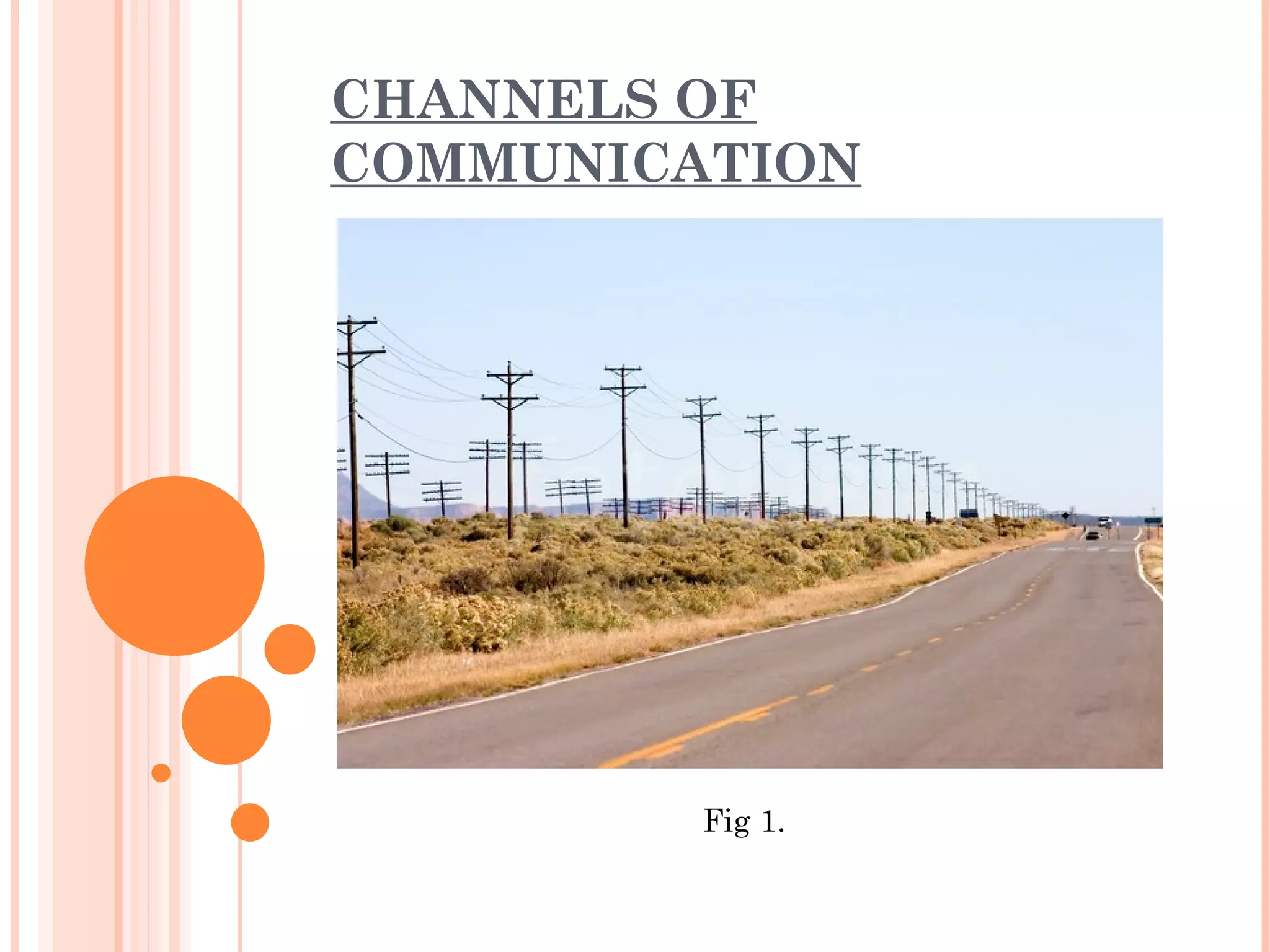
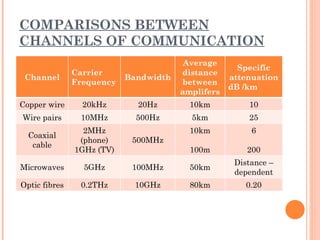
CHANNELS OF
COMMUNICATION


         Fig 1.
CHANNELS OF COMMUNICATION

Copper  wires
Wire pairs
Coaxial cables
Optic fibres
Radio waves
Microwaves
Satellites
COPPER WIRES


     Fig 2.
COPPER WIRES
 Cheap
 Used in the first telephone networks (1876) and
  still used today.
 Copper wires transmit electrical current.
 Current is not constant so produces variations in
  magnetic fields.
 Variations in magnetic field produce cross – talk.
 Cross – talk generates noise and interference.
 Copper wires need to be spaced apart to reduce
  effects.
 Low bandwidth (20kHz).
 Frequent need for amplification (every 10km).
WIRE PAIRS


             Fig 3.
WIRE PAIRS
 Twisted wires carry currents in opposite
  directions.
 Opposite currents reduces magnetic field
  interference.
 Twisted wires reduce flux linkage.

 Minimizing area minimizes unwanted signals
  created by electromagnetic induction due less
  exposure to other magnetic fields.
 Problems with attenuation. Amplification needed
  every 5km.
 Low bandwidth (500kHz).

 Distorts transmitted radio waves travelling in
  wire of different frequencies and speeds due to
  dispersion.
COAXIAL CABLE


            Fig 4.
COAXIAL CABLE
 Coaxial refers to the common axis of the two
  conductors. Both conductors are parallel.
 Most common cable for transmitting TV and
  video signals.
 Grounded shield protects core.
 Data is sent through central copper core.
 Electric and magnetic fields are confined within
  the dielectric.
 Interference from outside noise is reduced by
  outer shield, grounded shield and dielectric.
 Good at carrying weak signals.
 High bandwidth (500MHz)
 Amplification (MHz = 10km, GHz = 100m).
 Buried underground which is expensive.
OPTIC FIBRES


               Fig 4.
OPTIC FIBRES
 Replacing Coaxial cable
 High frequency signals (approaching THz)

 High bandwidth (10GHz)

 Low attenuation

 Amplification every 80km

 Perfect regeneration (Schmitt trigger)
RADIO SIGNALS


Fig 5


Fig 6
SURFACE RADIO WAVES


    Fig 7.


 Frequencies of 3MHz, wavelengths ≤ 100m
 Diffracted by Earth’s surface, therefore following
  the curvature of the Earth.
 AM radio transmissions can travel distances of
  100’s km.
 Powerful transmitters at low frequencies of 3kHz
  can travel 1000’s km.
SKY RADIO WAVES


                                                                  Fig 8


   Radio waves of 3MHz up to 30MHz.
   Radio waves suffer total internal reflection.
   Wave travels a certain distance from transmitter called
    ‘skip distance’.
   ‘Skip distance’ is unreliable due to changes in ionosphere.
   Severe problems with attenuation.
   Huge interference due to ions ionosphere.
SPACE RADIO WAVES


                                           Fig 9.


 Radio waves of frequencies above 30MHz.
 Waves travel in straight lines and are not
  effected by ionosphere (λ = 10m).
 Used for Earth bound satellite transmissions,
  FM transmissions and GPS.
MICROWAVES

                                                 Fig 10


   High frequency waves (GHz)
   Large bandwidth (100MHz)
   Multiplexing possible due to large bandwidth.
   Travel in straight lines, not effected by ionosphere.
   Reduced attenuation.
COMPARISONS BETWEEN
CHANNELS OF COMMUNICATION
                                        Average
                                                     Specific
               Carrier                 distance
 Channel                   Bandwidth               attenuation
               Frequency               between
                                                   dB /km
                                       amplifers
Copper wire      20kHz       20Hz        10km          10
Wire pairs      10MHz        500Hz       5km           25
                 2MHz                    10km           6
  Coaxial
                (phone)     500MHz
   cable
               1GHz (TV)                 100m          200
                                                    Distance –
Microwaves       5GHz       100MHz       50km
                                                    dependent
Optic fibres    0.2THz       10GHz       80km          0.20
SATELLITES


             Fig 11.
GEOSTATIONARY SATELLITES


   Equatorial orbit approximately 42000km above the Earth’s
    centre.
   Expensive to put into space (1963). However ideal for
    communication.
   Communication signals need to be in the range of GHz.
   Large bandwidth means multiplexing is possible.
   Limited power in satellite means that down-link signal
    transmission must require low power signals.
   Up-link signals need to be powerful and have higher
    frequencies than down-link signals.
GEOSTATIONARY SATELLITES


   13 equatorial countries, 7 have equatorial space. Who
    owns the space?
   1 geostationary satellite can cover 42% of the entire
    surface of the Earth.
   3 geostationary satellites can cover the entire surface,
    not taking into consideration the polar caps.
POLAR SATELLITES


Fig 14.


 Orbits poles a few hundred km’s above Earth
  surface.
 Can receive, store and retransmit data at a later
  time.
 Cheaper to put into orbit and requires less power
  to up-link signals.
 GPS
SATELLITES
 Communication to rural areas.
 Environmental concerns.

     No more cables but increasing space junk.
   International understanding.
    No international boundaries leading to international
    understanding. However there is always extremism
   Colonizing space.
HIGH BANDWIDTH
COMMUNICATION
Good points
 Multiple communications
 Sharing of information
 Business


Bad points
 Copyright infringement
 Extreme views
 Plagiarism
 Inappropriate material
 Spam
PHOTO URL’S
   Fig 1 -
    http://gb.fotolibra.com/images/previews/214705-telegraph-poles-route-66-near-bluewater-nm.jpeg
   Fig 2 -
    http://img.diytrade.com/cdimg/342538/1772020/0/1135589056/Single_Crystal_Copper_Wire.jpg
   Fig 3 -
    http://image.made-in-china.com/4f0j00kBYQraIyVWbt/Station-Wire-With-One-Twisted-Pair-Conductors
   Fig 4 - http://indolinkenglish.files.wordpress.com/2011/11/fiber-optic-cable-008.jpg
   Fig 5 -
    http://www.sciencephoto.com/image/345583/large/T3000586-Radio_masts_with_radio_waves-SPL.jpg
   Fig 6 - http://shariqa.com/E.M%20Wave%20Still.jpg
   Fig 7 - http://www.radio-electronics.com/info/propagation/ground_wave/ground_wave.gif
   Fig 8 - http://www.eoearth.org/files/155501_155600/155562/radio_transmissions.jpg
   Fig 9 - http://www.spaceweather.gc.ca/images/tech/effectsgps450.gif
   Fig 10 - http://zone.ni.com/cms/images/devzone/ph/ab273253214.gif
   Fig 11 - http://i.telegraph.co.uk/multimedia/archive/01514/SMOS_1514480c.jpg
   Fig 12- http://globalmicrowave.org/content/equitorial_orbit_geo.jpg
   Fig 13 - http://www.worldatlas.com/aatlas/newart/locator/equator.gif
   Fig 14 - http://globalmicrowave.org/content/polar_orbit.jpg
SOURCES OF REFERENCE
 Hamper, C. (2009). Higher Level Physics
  developed specifically for the IB Diploma . Essex:
  Pearson Education Limited.
 Tsokos, K.A. (2008). Physics for IB diploma, fifth
  addition. Cambridge: Cambridge University
  Press.

Channels of communication

  • 1.
  • 2.
    CHANNELS OF COMMUNICATION Copper wires Wire pairs Coaxial cables Optic fibres Radio waves Microwaves Satellites
  • 3.
  • 4.
    COPPER WIRES  Cheap Used in the first telephone networks (1876) and still used today.  Copper wires transmit electrical current.  Current is not constant so produces variations in magnetic fields.  Variations in magnetic field produce cross – talk.  Cross – talk generates noise and interference.  Copper wires need to be spaced apart to reduce effects.  Low bandwidth (20kHz).  Frequent need for amplification (every 10km).
  • 5.
  • 6.
    WIRE PAIRS  Twistedwires carry currents in opposite directions.  Opposite currents reduces magnetic field interference.  Twisted wires reduce flux linkage.  Minimizing area minimizes unwanted signals created by electromagnetic induction due less exposure to other magnetic fields.  Problems with attenuation. Amplification needed every 5km.  Low bandwidth (500kHz).  Distorts transmitted radio waves travelling in wire of different frequencies and speeds due to dispersion.
  • 7.
  • 8.
    COAXIAL CABLE  Coaxialrefers to the common axis of the two conductors. Both conductors are parallel.  Most common cable for transmitting TV and video signals.  Grounded shield protects core.  Data is sent through central copper core.  Electric and magnetic fields are confined within the dielectric.  Interference from outside noise is reduced by outer shield, grounded shield and dielectric.  Good at carrying weak signals.  High bandwidth (500MHz)  Amplification (MHz = 10km, GHz = 100m).  Buried underground which is expensive.
  • 9.
  • 10.
    OPTIC FIBRES  ReplacingCoaxial cable  High frequency signals (approaching THz)  High bandwidth (10GHz)  Low attenuation  Amplification every 80km  Perfect regeneration (Schmitt trigger)
  • 11.
  • 12.
    SURFACE RADIO WAVES Fig 7.  Frequencies of 3MHz, wavelengths ≤ 100m  Diffracted by Earth’s surface, therefore following the curvature of the Earth.  AM radio transmissions can travel distances of 100’s km.  Powerful transmitters at low frequencies of 3kHz can travel 1000’s km.
  • 13.
    SKY RADIO WAVES Fig 8  Radio waves of 3MHz up to 30MHz.  Radio waves suffer total internal reflection.  Wave travels a certain distance from transmitter called ‘skip distance’.  ‘Skip distance’ is unreliable due to changes in ionosphere.  Severe problems with attenuation.  Huge interference due to ions ionosphere.
  • 14.
    SPACE RADIO WAVES Fig 9.  Radio waves of frequencies above 30MHz.  Waves travel in straight lines and are not effected by ionosphere (λ = 10m).  Used for Earth bound satellite transmissions, FM transmissions and GPS.
  • 15.
    MICROWAVES Fig 10  High frequency waves (GHz)  Large bandwidth (100MHz)  Multiplexing possible due to large bandwidth.  Travel in straight lines, not effected by ionosphere.  Reduced attenuation.
  • 16.
    COMPARISONS BETWEEN CHANNELS OFCOMMUNICATION Average Specific Carrier distance Channel Bandwidth attenuation Frequency between dB /km amplifers Copper wire 20kHz 20Hz 10km 10 Wire pairs 10MHz 500Hz 5km 25 2MHz 10km 6 Coaxial (phone) 500MHz cable 1GHz (TV) 100m 200 Distance – Microwaves 5GHz 100MHz 50km dependent Optic fibres 0.2THz 10GHz 80km 0.20
  • 17.
    SATELLITES Fig 11.
  • 18.
    GEOSTATIONARY SATELLITES  Equatorial orbit approximately 42000km above the Earth’s centre.  Expensive to put into space (1963). However ideal for communication.  Communication signals need to be in the range of GHz.  Large bandwidth means multiplexing is possible.  Limited power in satellite means that down-link signal transmission must require low power signals.  Up-link signals need to be powerful and have higher frequencies than down-link signals.
  • 19.
    GEOSTATIONARY SATELLITES  13 equatorial countries, 7 have equatorial space. Who owns the space?  1 geostationary satellite can cover 42% of the entire surface of the Earth.  3 geostationary satellites can cover the entire surface, not taking into consideration the polar caps.
  • 20.
    POLAR SATELLITES Fig 14. Orbits poles a few hundred km’s above Earth surface.  Can receive, store and retransmit data at a later time.  Cheaper to put into orbit and requires less power to up-link signals.  GPS
  • 21.
    SATELLITES  Communication torural areas.  Environmental concerns. No more cables but increasing space junk.  International understanding. No international boundaries leading to international understanding. However there is always extremism  Colonizing space.
  • 22.
    HIGH BANDWIDTH COMMUNICATION Good points Multiple communications  Sharing of information  Business Bad points  Copyright infringement  Extreme views  Plagiarism  Inappropriate material  Spam
  • 23.
    PHOTO URL’S  Fig 1 - http://gb.fotolibra.com/images/previews/214705-telegraph-poles-route-66-near-bluewater-nm.jpeg  Fig 2 - http://img.diytrade.com/cdimg/342538/1772020/0/1135589056/Single_Crystal_Copper_Wire.jpg  Fig 3 - http://image.made-in-china.com/4f0j00kBYQraIyVWbt/Station-Wire-With-One-Twisted-Pair-Conductors  Fig 4 - http://indolinkenglish.files.wordpress.com/2011/11/fiber-optic-cable-008.jpg  Fig 5 - http://www.sciencephoto.com/image/345583/large/T3000586-Radio_masts_with_radio_waves-SPL.jpg  Fig 6 - http://shariqa.com/E.M%20Wave%20Still.jpg  Fig 7 - http://www.radio-electronics.com/info/propagation/ground_wave/ground_wave.gif  Fig 8 - http://www.eoearth.org/files/155501_155600/155562/radio_transmissions.jpg  Fig 9 - http://www.spaceweather.gc.ca/images/tech/effectsgps450.gif  Fig 10 - http://zone.ni.com/cms/images/devzone/ph/ab273253214.gif  Fig 11 - http://i.telegraph.co.uk/multimedia/archive/01514/SMOS_1514480c.jpg  Fig 12- http://globalmicrowave.org/content/equitorial_orbit_geo.jpg  Fig 13 - http://www.worldatlas.com/aatlas/newart/locator/equator.gif  Fig 14 - http://globalmicrowave.org/content/polar_orbit.jpg
  • 24.
    SOURCES OF REFERENCE Hamper, C. (2009). Higher Level Physics developed specifically for the IB Diploma . Essex: Pearson Education Limited.  Tsokos, K.A. (2008). Physics for IB diploma, fifth addition. Cambridge: Cambridge University Press.