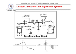
This document discusses topics related to discrete-time signals and systems from the textbook Discrete-Time Signal Processing by Alan V. Oppenheim and Ronald W. Schafer. It covers sampling of continuous-time signals to obtain discrete-time signals, basic discrete-time sequences and operations, discrete-time systems including linear and time-invariant systems, and examples such as the ideal delay system and moving average filter. Frequency characteristics of discrete-time signals such as periodicity are also examined.

![Discrete-Time Signal Processing, 2/E by Alan V. Oppenheim and Ronald W. Schafer
Chapter 2 Discrete
Chapter 2 Discrete-
-Time Signal and Systems
Time Signal and Systems
Xa(t): Analog signal
X[n]: discrete signal
Cos(ωn)= cos(Ωt)|t=nT
ΩT
ω=ΩT
ω: frequency of discrete signal
Ω: frequency of analog signal
q y g g
T: sampling interval 1/T=f = sampling frequency](https://image.slidesharecdn.com/ch2discretetimesignalandsystems-230606064019-94a62f87/85/Ch2_Discrete-time-signal-and-systems-pdf-7-320.jpg)
![Discrete-Time Signal Processing, 2/E by Alan V. Oppenheim and Ronald W. Schafer
Chapter 2 Discrete
Chapter 2 Discrete-
-Time Signal and Systems
Time Signal and Systems
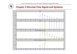
Figure 2.2 (a) Segment of a continuous-time speech signal xa(t ). (b) Sequence of samples x[n] = xa(nT ) obtained
g ( ) g p g a( ) ( ) q p [ ] a( )
from the signal in part (a) with T = 125 µs.](https://image.slidesharecdn.com/ch2discretetimesignalandsystems-230606064019-94a62f87/85/Ch2_Discrete-time-signal-and-systems-pdf-8-320.jpg)
![Discrete-Time Signal Processing, 2/E by Alan V. Oppenheim and Ronald W. Schafer
Chapter 2 Discrete
Chapter 2 Discrete-
-Time Signal and Systems
Time Signal and Systems
2.1.1 Basic Sequences and Sequence Operations
Delayed Sequence: y[n] = x[n-n0],
where n0 is a integer representing the delay
⎧ 0
0
Unit sample sequence (Dirac delta function):
⎩
⎨
⎧
=
≠
=
δ
0
n
,
1
0
n
,
0
]
n
[
Expression of a sequence using delta function:
Expression of a sequence using delta function:
Expression of a sequence using delta function:
Expression of a sequence using delta function:
∑
∞
δ ]
k
[
]
k
[
]
[ ∑
−∞
=
−
δ
=
k
]
k
n
[
]
k
[
x
]
n
[
x](https://image.slidesharecdn.com/ch2discretetimesignalandsystems-230606064019-94a62f87/85/Ch2_Discrete-time-signal-and-systems-pdf-9-320.jpg)
![Discrete-Time Signal Processing, 2/E by Alan V. Oppenheim and Ronald W. Schafer
Chapter 2 Discrete
Chapter 2 Discrete-
-Time Signal and Systems
Time Signal and Systems
Unit Step sequence:
The relation between unit function and delta function
The relation between unit function and delta function
]
[
]
1
[
]
[
]
[
]
1
[
]
1
[
]
[
∞
−
+
+
−
+
=
+
−
+
+
+
−∞
+
−∞
=
n
δ
n
δ
n
δ
n
δ
n
δ
δ
δ
K
K
∑
∑ −∞
=
∞
−∞
=
δ
=
−
⋅
δ
=
⎩
⎨
⎧
<
≥
=
n
k
k
]
k
[
]
k
n
[
u
]
k
[
0
n
,
0
0
n
,
1
]
n
[
u
equal)
are
equations
two
these
n,
number
finite
any
(for
If n-k ≥ 0, u[n-k]=1, then u[n-k]=1 exists when n≥k
Besides ]
1
n
[
u
]
n
[
u
]
n
[ −
−
=
δ
Besides, ]
1
n
[
u
]
n
[
u
]
n
[ =
δ
Impulse sequence:
Exponential and sinusoidal sequence (General form):](https://image.slidesharecdn.com/ch2discretetimesignalandsystems-230606064019-94a62f87/85/Ch2_Discrete-time-signal-and-systems-pdf-10-320.jpg)
![Discrete-Time Signal Processing, 2/E by Alan V. Oppenheim and Ronald W. Schafer
Chapter 2 Discrete
Chapter 2 Discrete-
-Time Signal and Systems
Time Signal and Systems
Sinusoidal sequences: )
n
cos(
A
]
n
[
x 0 φ
+
ω
= , for all n
⎧ ≥
α 0
n
A n
Recall the exponential sequence
⎩
⎨
⎧
<
≥
α
=
0
n
,
0
0
n
,
A
]
n
[
x
if 0
j
e
|
| ω
α
=
α And
φ
j
e
A
A |
|
1 = then
( ) ]
[
2
1
]
[
]
[
2
1 0
0
2
1
n
ω
j
φ
j
n
ω
j
φ
j
e
Ae
e
Ae
n
x
n
x −
−
+
=
+
=
, if e
|
| α
α And e
A
A |
|
1 , then
|
|
|
|
]
[
)
(
1
1
0
e
α
e
A
α
A
n
x n
ω
j
n
φ
j
n
=
=
)
sin(
|
|
|
|
)
cos(
|
|
|
|
|
|
|
|
0
0
)
( 0
φ
n
ω
α
A
j
φ
n
ω
α
A
e
α
A
n
n
φ
n
ω
j
n
+
⋅
+
+
⋅
=
⋅
= +
Especially,| α| =1
)
i (
|
|
)
(
|
|
]
[ A
j
A
Frequency phase
)
sin(
|
|
)
cos(
|
|
]
[ 0
0
1 φ
n
ω
A
j
φ
n
ω
A
n
x +
+
+
=
Complex exponential sequence
)
sin(
)
cos(
]
[ 0
0
1
2
2
0
φ
n
ω
A
j
φ
n
ω
A
e
α
e
A
α
A
n
x
α
n
ω
j
n
φ
j
n
+
−
+
=
=
=
=
−
−
−](https://image.slidesharecdn.com/ch2discretetimesignalandsystems-230606064019-94a62f87/85/Ch2_Discrete-time-signal-and-systems-pdf-11-320.jpg)
![Discrete-Time Signal Processing, 2/E by Alan V. Oppenheim and Ronald W. Schafer
Chapter 2 Discrete
Chapter 2 Discrete-
-Time Signal and Systems
Time Signal and Systems
In discrete signals, time index n is an integer which results in many important
differences from continuous-time sequences
differences from continuous time sequences.
Frequency periodicity:
n
j
n
2
j
n
j
n
)
2
(
j 0
0
0
Ae
e
Ae
Ae
]
n
[
x ω
π
ω
π
+
ω
=
=
=
]
n
cos[
A
]
n
)
r
2
cos[(
A
]
n
[
x φ
+
ω
=
φ
+
π
+
ω
= ]
n
cos[
A
]
n
)
r
2
cos[(
A
]
n
[
x 0
0 φ
+
ω
=
φ
+
π
+
ω
=
Time periodicity:
Time periodicity holds only when the following relation exits,
p y y g ,
]
N
n
[
x
]
n
[
x +
=
For sinusoid signals, Acos(ω0n+φ)=Acos(ω0n+ω0N+φ)
ω0N=2πk](https://image.slidesharecdn.com/ch2discretetimesignalandsystems-230606064019-94a62f87/85/Ch2_Discrete-time-signal-and-systems-pdf-12-320.jpg)
![Discrete-Time Signal Processing, 2/E by Alan V. Oppenheim and Ronald W. Schafer
Chapter 2 Discrete
Chapter 2 Discrete-
-Time Signal and Systems
Time Signal and Systems
ω=ΩT
Ω↑ then ω↑
Example 2.1
In continuous signals, signals with higher frequency usually
have shorter repetition period but this doesn’t hold in
have shorter repetition period, but this doesn t hold in
discrete signals.
),
4
/
cos(
]
[
1 n
n
x π
= N=8
),
8
/
3
cos(
]
[
2 n
n
x π
= N=16](https://image.slidesharecdn.com/ch2discretetimesignalandsystems-230606064019-94a62f87/85/Ch2_Discrete-time-signal-and-systems-pdf-13-320.jpg)
![Discrete-Time Signal Processing, 2/E by Alan V. Oppenheim and Ronald W. Schafer
Chapter 2 Discrete
Chapter 2 Discrete-
-Time Signal and Systems
Time Signal and Systems
2.2 Discrete
2.2 Discrete-
-Time Systems
Time Systems
x[n] y[n]
{ }
⋅
T
]}
n
[
x
{
T
]
n
[
y =
Example 2 2 The ideal delay system
Example 2.2 The ideal delay system
y[n] = x[n-nd],
where n is a fixed positive integer called the delay of the system
where nd is a fixed positive integer called the delay of the system.](https://image.slidesharecdn.com/ch2discretetimesignalandsystems-230606064019-94a62f87/85/Ch2_Discrete-time-signal-and-systems-pdf-14-320.jpg)
![Discrete-Time Signal Processing, 2/E by Alan V. Oppenheim and Ronald W. Schafer
Chapter 2 Discrete
Chapter 2 Discrete-
-Time Signal and Systems
Time Signal and Systems
Example 2.3 Moving Average
The general moving average system is defined by the equation
{ }
1
]
[
1
1
]
[
2
1
2
1
k
n
x
M
M
n
y
M
M
k
=
−
+
+
= ∑
−
=
{ }
]
[
]
[
]
1
[
]
[
1
1
2
1
1
2
1
M
n
x
n
x
M
n
x
M
n
x
M
M
−
+
+
+
+
−
+
+
+
+
+
= L
L
Figure 2.7 Sequence values involved in computing a moving average with M1 = 0 and M2 = 5.](https://image.slidesharecdn.com/ch2discretetimesignalandsystems-230606064019-94a62f87/85/Ch2_Discrete-time-signal-and-systems-pdf-15-320.jpg)
![Discrete-Time Signal Processing, 2/E by Alan V. Oppenheim and Ronald W. Schafer
Chapter 2 Discrete
Chapter 2 Discrete-
-Time Signal and Systems
Time Signal and Systems
2.2.1
2.2.1 Memoryless
Memoryless Systems
Systems
A system is referred to as memoryless if the output y[n] at every value of n
depends only on the input x[n] at the same value of n
Example 2.4
y[n] = (x[n])2 for all value of n
depends only on the input x[n] at the same value of n.
y[n] = (x[n]) , for all value of n
2.2.2 Linear Systems
2.2.2 Linear Systems
The class of linear systems is defined by the principle of superposition. If y1[n]
Additivity property
and y2[n] are the responses of a system when x1[n] and x2[n] are the respective
inputs, then the system is linear if and only if
]}
[
{
]}
[
{
]}
[
]
[
{ n
x
T
n
x
T
n
x
n
x
T +
+
Additivity property
Scaling or Homogeneity
property
]}
[
{
]}
[
{
]}
[
]
[
{ 2
1
2
1 n
x
T
n
x
T
n
x
n
x
T +
=
+
]
[
]}
[
{
]}
[
{ n
ay
n
x
aT
n
ax
T =
=
property
where a is an arbitrary constant. The first property is the additivity property, and
the second is the homogeneity or scaling property. These two properties together
comprise the principle of superposition stated as
comprise the principle of superposition, stated as
]}
[
{
]}
[
{
]}
[
]
[
{ 2
1
2
1 n
x
bT
n
x
aT
n
bx
n
ax
T +
=
+](https://image.slidesharecdn.com/ch2discretetimesignalandsystems-230606064019-94a62f87/85/Ch2_Discrete-time-signal-and-systems-pdf-16-320.jpg)
![Discrete-Time Signal Processing, 2/E by Alan V. Oppenheim and Ronald W. Schafer
Chapter 2 Discrete
Chapter 2 Discrete-
-Time Signal and Systems
Time Signal and Systems
For a linear system with arbitrary constants a and b, the
expression of generalized to the superposition of many inputs.
g y
]
n
[
x
a
]
n
[
x k
k
k
∑
=
Output of a linear system will be
General form:
]
n
[
y
b
]
n
[
y k
k
k
∑
=
p y
}
]
n
[
x
a
{
T
]
n
[
y
b
m k
k
k
m
m
∑ ∑
=
E l 2 5 Th l t t
n
Example 2.5 The accumulator system
∑
−∞
=
=
k
]
k
[
x
]
n
[
y Is linear?
Let x3 [n] = ax1[n]+bx2[n] and check the output is y3[n] = ay1[n]+by2[n] ?
])
k
[
bx
]
k
[
ax
(
]
k
[
x
]
n
[
y
n n
n
k
n
k
2
1
3
3 +
=
= ∑ ∑
−∞
= −∞
=
]
n
[
by
]
n
[
ay
]
k
[
x
b
]
k
[
x
a 2
1
k k
2
1 +
=
+
= ∑ ∑
−∞
= −∞
= Linear](https://image.slidesharecdn.com/ch2discretetimesignalandsystems-230606064019-94a62f87/85/Ch2_Discrete-time-signal-and-systems-pdf-17-320.jpg)
![Discrete-Time Signal Processing, 2/E by Alan V. Oppenheim and Ronald W. Schafer
Chapter 2 Discrete
Chapter 2 Discrete-
-Time Signal and Systems
Time Signal and Systems
Example 2.6 A Nonlinear System
Consider the system defined by
|).
]
[
(|
log
]
[ 10 n
x
n
w =
This system is not linear. For x1[n]=1 and x2[n] = 10, then
.
1
)
10
(
log
)
1
(
log
)
11
(
log
)
10
1
(
log 10
10
10
10 =
+
≠
=
+
Also, we have x2[n] = 10 .x1[n], but
1
)
10
1
(
l
]
[
0
)
1
(
log
]
[ 10
1 ≠
=
=
n
w
.
1
)
10
1
(
log
]
[ 10
2 =
⋅
=
n
w](https://image.slidesharecdn.com/ch2discretetimesignalandsystems-230606064019-94a62f87/85/Ch2_Discrete-time-signal-and-systems-pdf-18-320.jpg)
![Discrete-Time Signal Processing, 2/E by Alan V. Oppenheim and Ronald W. Schafer
Chapter 2 Discrete
Chapter 2 Discrete-
-Time Signal and Systems
Time Signal and Systems
2.2.3 Time
2.2.3 Time-
-Invariant Systems
Invariant Systems
A time-invariant system (equivalently often referred to as a shift-invariant system)
is one for with a time shift or delay of the input sequence causes a corresponding
is one for with a time shift or delay of the input sequence causes a corresponding
shift in the output sequence. Specifically, suppose that a system transforms the
input sequence with values x[n] into the output sequence with values y[n]. The
system is said to be time-invariant if for all n0 the input sequence with values x1[n]
system is said to be time invariant if for all n0 the input sequence with values x1[n]
= x[n-n0] produces the output sequence with values y1[n] = y[n-n0].
Example 2.7 The Accumulator as a Time –Invariant System
Consider the accumulator from Example 2.5. We define x1[n]= x[n-n0]. To
show time invariance, we solve for both y[n-n0] and y1[n] and compare them
to see whether they are equal. Therefore, setting a system T{.}, we have
y q g y { }
.
]
[
]
[
]}
[
{
]
[
]}
[
{
]
[ 0
1
1
1 ∑
∑ −∞
=
−∞
=
−
=
=
=
=
n
k
n
k
n
k
x
k
x
n
x
T
n
y
and
n
x
T
n
y
,
]
[
]
[ 0
0
∑
−
−∞
=
+
=
=
−
n
0
n
n
k
then
n
k
k'
setting
and
k
x
n
n
y
g
Considerin
.
]
'
[
]
[
'
0
0 ∑
−∞
=
−
=
−
n
k
n
k
x
n
n
y](https://image.slidesharecdn.com/ch2discretetimesignalandsystems-230606064019-94a62f87/85/Ch2_Discrete-time-signal-and-systems-pdf-19-320.jpg)
![Discrete-Time Signal Processing, 2/E by Alan V. Oppenheim and Ronald W. Schafer
Chapter 2 Discrete
Chapter 2 Discrete-
-Time Signal and Systems
Time Signal and Systems
Example 2.8 The Compressor System
Th t d fi d b th l ti
The system defined by the relation
with M a positive integer, is called a compressor. Specifically, it discards (M-1)
samples out of M; i e it creates the output sequence by selecting every Mth
.
n
-
Mn
x
n
y ∞
<
<
∞
= ],
[
]
[
samples out of M; i.e., it creates the output sequence by selecting every Mth
sample. The system is not time-invariant, the output of the system when the
input is x1[n] must be equal to y[n-n0]. The output y1[n] that results from the
input x1[n] can be directly computed to be
input x1[n] can be directly computed to be
)]
(
[
]
[
]
[
].
[
]
[
0
0
0
1
n
n
M
x
n
n
y
n
y
condition,
delay
output
to
Compared
n
Mn
x
n
y
have
we
condition,
delay
input
For
2 −
=
−
=
−
=
Time-invariant is not compressible.
].
[n
y1
≠](https://image.slidesharecdn.com/ch2discretetimesignalandsystems-230606064019-94a62f87/85/Ch2_Discrete-time-signal-and-systems-pdf-20-320.jpg)
![Discrete-Time Signal Processing, 2/E by Alan V. Oppenheim and Ronald W. Schafer
Chapter 2 Discrete
Chapter 2 Discrete-
-Time Signal and Systems
Time Signal and Systems
2.2.4 Causality
2.2.4 Causality
A system is causal if for every choice of n the output sequence value at the
A system is causal if, for every choice of n0, the output sequence value at the
index n = n0 depends only on the input sequence values for n ≤ n0.
For example, Example 2.4 is causal if –M1 ≥ 0 and M2 ≥ 0.
Example 2.9 The Forward and Backward Difference Systems
The forward difference system is defined by the relation
y y
y[n] = x[n+1] – x[n].
Obviously y[n] depends on x[n+1]; therefore, the system is noncausal.
However, the backward difference system, defined by
y[n] = x[n] – x[n-1]
is causal.](https://image.slidesharecdn.com/ch2discretetimesignalandsystems-230606064019-94a62f87/85/Ch2_Discrete-time-signal-and-systems-pdf-21-320.jpg)
![Discrete-Time Signal Processing, 2/E by Alan V. Oppenheim and Ronald W. Schafer
Chapter 2 Discrete
Chapter 2 Discrete-
-Time Signal and Systems
Time Signal and Systems
2.2.5 Stability
2.2.5 Stability
A system is stable in the bounded-input bounded-output (BIBO) sense if and
only if every bounded input sequence produces a bounded output sequence The
only if every bounded input sequence produces a bounded output sequence. The
input x[n] is bounded if there exits a fixed positive finite value Bx such that
|x[n]| ≦Bx ≦ ∞ for all n.
Stability requires that for every bounded input there exists a fixed positive finite
Stability requires that for every bounded input there exists a fixed positive finite
value By such that
|y[n]| ≦By ≦ ∞ for all n.
Example 2.10 Testing for Stability or Instability
(i) Ex 2.4. For |x[n]| ≦Bx , then |y[n]| = |x[n]|2≦ Bx2
(ii) E 2 6 F [ ] 0 [ ] l (| [ ]|)
(ii) Ex 2.6. For x[n] = 0, y[n] = log10(|x[n]|) = - ∞
(iii) Ex. 2.5. For x[n] = u[n] with Bx =1,
∑ ⎨
⎧ <
n
0
n
k
,
0
]
[
]
[
Ans: (i) stable
∑
−∞
=
⎩
⎨
≥
+
=
=
k
0
n
n
k
u
n
y
,
1
]
[
]
[
Ans: (i) stable
(ii) not stable
(iii) not stable](https://image.slidesharecdn.com/ch2discretetimesignalandsystems-230606064019-94a62f87/85/Ch2_Discrete-time-signal-and-systems-pdf-22-320.jpg)
![Discrete-Time Signal Processing, 2/E by Alan V. Oppenheim and Ronald W. Schafer
Chapter 2 Discrete
Chapter 2 Discrete-
-Time Signal and Systems
Time Signal and Systems
2.3 Linear Time
2.3 Linear Time-
-Invariant systems
Invariant systems
A particularly important class of systems consists of those that are linear and
time invariant. This class of systems has significant signal-processing
applications.
Let hk[n] be the response of the system to δ[n-k], an impulse occurring at
e k[ ] be e espo se o e sys e o δ[ ], a pu se occu g a
n=k.
∑
∞
−∞
=
−
δ
=
k
]}
k
n
[
]
k
[
x
{
T
]
n
[
y
Time invariant
∑ ∑
∑
∞
−∞
=
∞
−∞
=
∞
−∞
=
=
−
=
−
δ
=
k k
k
k
]
n
[
h
]
k
[
x
]
k
n
[
h
]
k
[
x
]}
k
n
[
{
T
]
k
[
x
h[n] with k delayed input
Linearity
h[n] with k delayed input
(T{.} is LTI system)
Define:
Convolution sum:
Convolution sum: y[n] = x[n]
y[n] = x[n] ∗
∗ h[n]
h[n]](https://image.slidesharecdn.com/ch2discretetimesignalandsystems-230606064019-94a62f87/85/Ch2_Discrete-time-signal-and-systems-pdf-23-320.jpg)
![Discrete-Time Signal Processing, 2/E by Alan V. Oppenheim and Ronald W. Schafer
Chapter 2 Discrete
Chapter 2 Discrete-
-Time Signal and Systems
Time Signal and Systems
y[n] = x[n]
y[n] = x[n] ∗
∗ h[n]
h[n]
Sum
Sum
∑
∞
−∞
=
−
⋅
=
k
]
k
n
[
h
]
k
[
x
]
n
[
y
volution
volution
of
Conv
of
Conv
example
example
An
e
An
e
Figure 2.8 Representation of the output of an LTI
system as the superposition of responses to
system as the superposition of responses to
individual samples of the input.](https://image.slidesharecdn.com/ch2discretetimesignalandsystems-230606064019-94a62f87/85/Ch2_Discrete-time-signal-and-systems-pdf-24-320.jpg)
![Discrete-Time Signal Processing, 2/E by Alan V. Oppenheim and Ronald W. Schafer
Chapter 2 Discrete
Chapter 2 Discrete-
-Time Signal and Systems
Time Signal and Systems
It is worthy to note that the term h[n-k] in convolution sum also can be
represented as h[-(k-n)]. Therefore, ∞
∞
( )
∑
∑
∞
∞
−
∞
−∞
=
−
−
⋅
=
−
⋅
= )]
n
k
(
[
h
]
k
[
x
]
k
n
[
h
]
k
[
x
]
n
[
y
k
h[k]
h[k]
h[
h[-
-k] = h[0
k] = h[0-
-k]
k]
h[
h[ k] h[0
k] h[0 k]
k]
h[n
h[n-
-k] = h[
k] = h[-
-(k
(k-
-n)]
n)]
Figure 2.9 Forming the sequence h[n − k]. (a) The sequence h[k] as a function of k. (b) The sequence h[−k] as a
function of k. (c) The sequence h[n − k] = h[ − (k − n)] as a function of k for n = 4.](https://image.slidesharecdn.com/ch2discretetimesignalandsystems-230606064019-94a62f87/85/Ch2_Discrete-time-signal-and-systems-pdf-25-320.jpg)
![Discrete-Time Signal Processing, 2/E by Alan V. Oppenheim and Ronald W. Schafer
Chapter 2 Discrete
Chapter 2 Discrete-
-Time Signal and Systems
Time Signal and Systems
Example 2.11 Analytical Evaluation of Convolution sum
Example 2.11 Analytical Evaluation of Convolution sum
Consider a system with impulse response
y p p
⎩
⎨
⎧ −
≤
≤
=
−
−
=
otherwise
,
0
1
N
n
0
,
1
]
N
n
[
u
]
n
[
u
]
n
[
h
⎩
0 N-1
The input is ]
n
[
u
a
]
n
[
x n
=
∞
∑
∞
∞
−
−
−
⋅
= )]
n
k
(
[
h
]
k
[
x
]
n
[
y](https://image.slidesharecdn.com/ch2discretetimesignalandsystems-230606064019-94a62f87/85/Ch2_Discrete-time-signal-and-systems-pdf-26-320.jpg)
![Discrete-Time Signal Processing, 2/E by Alan V. Oppenheim and Ronald W. Schafer
Ans:
Figure 2.10 Sequence involved in computing a discrete convolution.
(a)–(c) The sequences x[k] and h[n− k] as a function of k for different
values of n. (Only nonzero samples are shown.) (d) Corresponding
output sequence as a function of n.](https://image.slidesharecdn.com/ch2discretetimesignalandsystems-230606064019-94a62f87/85/Ch2_Discrete-time-signal-and-systems-pdf-27-320.jpg)
![Discrete-Time Signal Processing, 2/E by Alan V. Oppenheim and Ronald W. Schafer
Bounded Input is not guaranteed for Bounded Output
(The requirement for a stable system)
∞
(The requirement for a stable system)
Linear time-invariant systems are stable if and only if the impulse
response is absolutely summable, i.e., if
∑
∞
−∞
=
∞
<
=
k
|
]
k
[
h
|
S Sufficient
Sufficient condition for stability
condition for stability
∑
∑
∞
−∞
=
∞
−∞
=
−
≤
−
=
k
k
|
]
k
n
[
x
||
]
k
[
h
|
]
k
n
[
x
]
k
[
h
|
]
n
[
y
|
B
|
]
n
[
x
| ≤
If x[n] is bounded so that x
B
|
]
n
[
x
| ≤
If x[n] is bounded, so that
∑
∞
≤ x |
]
k
[
h
|
B
|
]
n
[
y
|
Consider:
Th [ ] i l l
−∞
=
k
⎪
⎨
⎧
≠
−
=
0
]
n
[
h
,
|
]
n
[
h
|
]
n
[
h
]
n
[
x
*
The sequence x[n] is clearly
bounded to unity. However,
the value of the output at
n=0 is:
⎪
⎩
⎨
=
−
=
0
]
n
[
h
,
0
|
]
n
[
h
|
]
n
[
x
∑ ∑
∞ ∞ 2
S
|
]
k
[
h
|
]
k
[
h
]
k
[
]
0
[
n=0 is:
Bounded input produce unbounded output
Bounded input produce unbounded output
∑ ∑
−∞
= −∞
=
=
=
−
=
k k
S
|
]
k
[
h
|
|
]
[
|
]
k
[
h
]
k
[
x
]
0
[
y](https://image.slidesharecdn.com/ch2discretetimesignalandsystems-230606064019-94a62f87/85/Ch2_Discrete-time-signal-and-systems-pdf-30-320.jpg)
![Discrete-Time Signal Processing, 2/E by Alan V. Oppenheim and Ronald W. Schafer
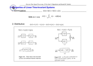
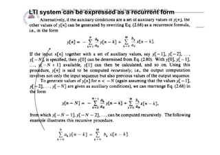
The expression of equivalent LTI systems (example 1)
noncausal
noncausal
causal
causal
Figure 2.12 (a) Cascade combination of two
LTI systems. (b) Equivalent cascade. (c)
]
1
[
])
[
]
1
[
(
]
[
h δ
δ
δ
y ( ) q ( )
Single equivalent system.
])
n
[
]
1
n
[
(
]
1
n
[
]
1
n
[
])
n
[
]
1
n
[
(
]
n
[
h
δ
−
+
δ
∗
−
δ
=
−
δ
∗
δ
−
+
δ
=
]
1
n
[
]
n
[ −
δ
−
δ
=](https://image.slidesharecdn.com/ch2discretetimesignalandsystems-230606064019-94a62f87/85/Ch2_Discrete-time-signal-and-systems-pdf-32-320.jpg)
![Discrete-Time Signal Processing, 2/E by Alan V. Oppenheim and Ronald W. Schafer
Chapter 2 Discrete
Chapter 2 Discrete-
-Time Signal and Systems
Time Signal and Systems
2.5 Linear constant
2.5 Linear constant-
-coefficient Differenece Equations
coefficient Differenece Equations
Nth order linear constant coefficient difference equation:
Nth-order linear constant-coefficient difference equation:
∑ ∑
= =
−
=
−
N
0
k
M
0
m
m
k ]
m
n
[
x
b
]
k
n
[
y
a
∑ ∑
∞
−
⋅
=
=
= 1
n
1 ],
k
n
[
h
]
k
[
x
]
n
[
h
*
]
n
[
x
]
k
[
x
]
n
[
y
Example 2.12
Example 2.12
Consider:
0
k 0
m
∑
∑ ∑
−∞
=
∞
− ∞
−
δ
=
n
k
1
1
1
]
k
[
]
n
[
h
where
],
k
n
[
h
]
k
[
x
]
n
[
h
]
n
[
x
]
k
[
x
]
n
[
y
Consider:
∞
=
k
Input y[n] into a inverse system
Y[n] Inverse system ?
]
1
n
[
]
n
[
]
n
[
h2 −
δ
−
δ
=
Inverse system:
]
n
[
h
*
]
n
[
y
]
n
[
x ]
n
[
h
*
]
n
[
y
]
n
[
x 2
=](https://image.slidesharecdn.com/ch2discretetimesignalandsystems-230606064019-94a62f87/85/Ch2_Discrete-time-signal-and-systems-pdf-34-320.jpg)
![Discrete-Time Signal Processing, 2/E by Alan V. Oppenheim and Ronald W. Schafer
Chapter 2 Discrete
Chapter 2 Discrete-
-Time Signal and Systems
Time Signal and Systems
∑
=
n
k
]
k
[
x
]
n
[
y
Y[n]
X[n]
−∞
=
k
∑
−
=
−
1
n
]
k
[
x
]
1
n
[
y One-sample
Y[n]
[ ]
∑
−∞
=
k
]
[
]
[
y
∑
−1
n
One-sample
delay
Y[n-1]
∑
−∞
=
+
=
k
]
k
[
x
]
n
[
x
]
n
[
y
Y[n 1]
]
1
n
[
y
]
n
[
x
]
n
[
y −
+
= ]
n
[
x
]
1
n
[
y
]
n
[
y =
−
−](https://image.slidesharecdn.com/ch2discretetimesignalandsystems-230606064019-94a62f87/85/Ch2_Discrete-time-signal-and-systems-pdf-35-320.jpg)
![Discrete-Time Signal Processing, 2/E by Alan V. Oppenheim and Ronald W. Schafer
Chapter 2 Discrete
Chapter 2 Discrete-
-Time Signal and Systems
Time Signal and Systems
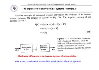
Example 2.13 Difference equation representation of the moving
Example 2.13 Difference equation representation of the moving-
-average system
average system
])
1
M
n
[
u
]
n
[
u
(
)
1
M
(
1
]
n
[
h 2
2
−
−
−
+
=
Consider causal moving-average
system with M1=0,
∑ −
=
=
2
M
]
k
n
[
x
)
1
M
(
1
]
n
[
h
*
]
n
[
x
]
n
[
y ∑
=
+ 0
k
2 )
1
M
(
]}
n
[
u
*
])
1
M
n
[
]
n
[
{(
)
1
M
(
1
]
n
[
h 2
2
−
−
δ
−
δ
+
=
]
n
[
u
*
])
1
M
n
[
x
]
n
[
x
(
)
1
M
(
1
]
n
[
h
*
]
n
[
x
]
n
[
y 2
2
−
−
−
+
=
=](https://image.slidesharecdn.com/ch2discretetimesignalandsystems-230606064019-94a62f87/85/Ch2_Discrete-time-signal-and-systems-pdf-36-320.jpg)
![Discrete-Time Signal Processing, 2/E by Alan V. Oppenheim and Ronald W. Schafer
Chapter 2 Discrete
Chapter 2 Discrete-
-Time Signal and Systems
Time Signal and Systems
2.6 Frequency Domain Representation of Discrete
2.6 Frequency Domain Representation of Discrete-
-Time Signal and
Time Signal and Systems
Systems
2.6.1 Eigen functions for Linear Time
2.6.1 Eigen functions for Linear Time-
-Invariant Systems
Invariant Systems
Input sequence x[n] = ejwn is a set of eigen-function to represent the
frequency response of h[n]
e
]
k
[
h
]
k
n
[
x
]
k
[
h
]
n
[
x
*
]
n
[
h
]
n
[
y )
k
n
(
j
∑
∑
∞
−
ω
∞
=
=
=
}
e
]
k
[
h
{
e
e
]
k
[
h
]
k
n
[
x
]
k
[
h
]
n
[
x
*
]
n
[
h
]
n
[
y
k
j
n
j
k
)
(
j
k
∑
∑
∑
∞
ω
−
ω
−∞
=
−∞
=
=
=
−
⋅
=
=
}
e
]
k
[
h
{
e
k
∑
−∞
=
=
∑
∞
ω
−
ω
= k
j
j
e
]
k
[
h
)
e
(
H
If we define , then
n
j
j
e
)
e
(
H
]
n
[
y ω
ω
=
∑
−∞
=
k
]
[
)
(
If we define , t e )
(
]
[
y
Eigenfunction
j
j
j )
e
(
H
j
j
j j
|
)
(
H
|
)
(
H
ω
∠
ω
ω
Polar
Polar
form
form
)
e
(
jH
)
e
(
H
)
e
(
H j
I
j
R
j ω
ω
ω
+
=
)
e
(
H
j
j
j j
e
|
)
e
(
H
|
)
e
(
H ∠
ω
ω
=
form
form](https://image.slidesharecdn.com/ch2discretetimesignalandsystems-230606064019-94a62f87/85/Ch2_Discrete-time-signal-and-systems-pdf-38-320.jpg)
![Discrete-Time Signal Processing, 2/E by Alan V. Oppenheim and Ronald W. Schafer
Chapter 2 Discrete
Chapter 2 Discrete-
-Time Signal and Systems
Time Signal and Systems
Example 2.14 Frequency response of the ideal delay system
Example 2.14 Frequency response of the ideal delay system
Consider a ideal delay system defined by y[n]= x[n-nd] , where nd is a fixed
integer. If we consider
x[n]=ejωn as input to this system, then we have
y[n] = ejω(n-nd) = e-jωnd ejωn.
The frequency response of the ideal delay is therefore
H(ejω) = e-jωnd
An alternative way to obtain the frequency response is to compute the H(ejω)
i F i t f
using Fourier transform
∑
∞
∞
−
ω
−
ω
−
δ
= n
j
d
j
e
]
n
n
[
)
e
(
H
From the Euler relation the real and imaginary parts are
From the Euler relation, the real and imaginary parts are
)
n
cos(
)
e
(
H d
j
R ω
=
ω Polar form
Polar form
j
|
)
e
(
H
| =
ω
1
)
n
sin(
)
e
(
H d
j
I ω
=
ω
d
j
n
)
e
(
H
|
)
(
|
ω
−
=
∠ ω](https://image.slidesharecdn.com/ch2discretetimesignalandsystems-230606064019-94a62f87/85/Ch2_Discrete-time-signal-and-systems-pdf-39-320.jpg)
![Discrete-Time Signal Processing, 2/E by Alan V. Oppenheim and Ronald W. Schafer
Chapter 2 Discrete
Chapter 2 Discrete-
-Time Signal and Systems
Time Signal and Systems
*
*For any input signal, x[n], if the input signal can be represented as
n
j
k
k
n
e
]
n
[
x ω
∑α
=
Then from the principle of superposition the corresponding output of a
Then, from the principle of superposition, the corresponding output of a
linear time-invariant system is
n
j
j
k
k
k
e
)
e
(
H
]
n
[
y ω
ω
∑α
=
k
k )
(
]
[
y ∑
Thus if we can find a representation of x[n] as a superposition of ocmplex
Thus, if we can find a representation of x[n] as a superposition of ocmplex
exponential sequences, then we can find the output as aforementioned
equation if we know the frequency response of the system.](https://image.slidesharecdn.com/ch2discretetimesignalandsystems-230606064019-94a62f87/85/Ch2_Discrete-time-signal-and-systems-pdf-40-320.jpg)
![Discrete-Time Signal Processing, 2/E by Alan V. Oppenheim and Ronald W. Schafer
Chapter 2 Discrete
Chapter 2 Discrete-
-Time Signal and Systems
Time Signal and Systems
Example 2.15 Sinusoidal response of LTI system
Example 2.15 Sinusoidal response of LTI system
Since it is simple to express a sinusoid as a linear combination of complex
n
j
j
n
j
j
e
e
A
e
e
A
)
n
cos(
A
]
n
[
x 0
0
2
2
0
ω
−
φ
−
ω
φ
+
=
φ
+
ω
=
exponentials, let us consider a sinusoidal input
X1[n] X2[n]
The responses to x1[n] and x2[n] are y1[n] and y2[n].
A n
j
j
n
j
e
e
A
)
e
(
H
]
n
[
y 0
0
2
1 ω
φ
ω
=
n
j
j
n
j
e
e
A
)
e
(
H
]
n
[
y 0
0
2
2 ω
−
φ
−
ω
−
= )
(
]
[
y
2
]
e
e
)
e
(
H
e
e
)
e
(
H
[
A
]
n
[
y
]
n
[
y
]
n
[
y n
j
j
n
j
n
j
j
n
j 0
0
0
0
2
2
1 ω
−
φ
−
ω
−
ω
φ
ω
+
=
+
=
If h[ ] i l ill h l t th t H( j 0) H*( j 0) hi h i th t
If h[n] is real, we will show later that H(ejω0)=H*(e-jω0) which gives that
)
n
cos(
|
)
e
(
H
|
A
]
n
[
y n
j
θ
+
φ
+
ω
= ω
0
0
, where )
e
(
H j 0
ω
∠
=
θ](https://image.slidesharecdn.com/ch2discretetimesignalandsystems-230606064019-94a62f87/85/Ch2_Discrete-time-signal-and-systems-pdf-41-320.jpg)
![Discrete-Time Signal Processing, 2/E by Alan V. Oppenheim and Ronald W. Schafer
Chapter 2 Discrete
Chapter 2 Discrete-
-Time Signal and Systems
Time Signal and Systems
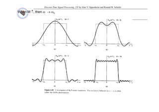
An important characteristic of discrete-time linear time-invariant
systems is of its periodicity of the variable ω with period 2π.
Consider
∑
∑
∞
−∞
=
ω
−
∞
−∞
=
π
+
ω
−
π
+
ω
=
=
n
n
j
n
n
)
2
(
j
n
)
2
(
j
e
]
n
[
h
e
]
n
[
h
)
e
(
H
n
j
n
2
j
n
j
n
)
2
(
j
e
e
e
e ω
−
π
−
ω
−
π
+
ω
−
=
=
)
(
)
( j
n
)
2
(
j ω
π
+
ω
)
e
(
H
)
e
(
H j
n
)
2
(
j ω
π
+
ω
=
Th f bt i H(
Th f bt i H( j
jω
ω) i i di ith i d
) i i di ith i d 2
2
Therefore, we obtain H(e
Therefore, we obtain H(ej
jω
ω) is periodic with period
) is periodic with period 2
2π
π.
.](https://image.slidesharecdn.com/ch2discretetimesignalandsystems-230606064019-94a62f87/85/Ch2_Discrete-time-signal-and-systems-pdf-42-320.jpg)
![Discrete-Time Signal Processing, 2/E by Alan V. Oppenheim and Ronald W. Schafer
Chapter 2 Discrete
Chapter 2 Discrete-
-Time Signal and Systems
Time Signal and Systems
Example 2.16 Frequency response of the moving
Example 2.16 Frequency response of the moving-
-averaging system
averaging system
⎧ ≤
≤ M
n
M
1 2
M
1
⎩
⎨
⎧ ≤
≤
−
= +
+
otherwise
,
0
M
n
M
,
]
n
[
h 2
1
1
M
M
1
2
1
∑
−
=
ω
−
ω
+
+
=
2
1
M
M
n
n
j
2
1
j
e
1
M
M
1
)
e
(
H
Frequency response
Frequency response
q y p
q y p
)
1
( 2
1
1 M
j
M
j
e
e +
− ω
ω )
(
2
1
2
1
1
1
1
)
( j
j
j
j
e
e
e
M
M
e
H −
−
−
+
+
= ω
ω
2
/
)
(
2
/
2
/
2
/
)
1
(
2
/
)
1
(
2
1
1
2
2
1
2
1
1
1 M
M
j
j
j
M
M
j
M
M
j
e
e
e
e
e
M
M
−
−
−
+
+
−
+
+
−
−
+
+
= ω
ω
ω
ω
ω
2
/
)
(
2
1
2
1
1
2
)
2
/
i (
]
2
/
)
1
(
sin[
1
1
1
M
M
j
e
M
M
M
M
e
e
M
M
−
−
+
+
=
+
+
ω
ω
2
1 )
2
/
sin(
1
M
M +
+ ω](https://image.slidesharecdn.com/ch2discretetimesignalandsystems-230606064019-94a62f87/85/Ch2_Discrete-time-signal-and-systems-pdf-44-320.jpg)
![Discrete-Time Signal Processing, 2/E by Alan V. Oppenheim and Ronald W. Schafer
Chapter 2 Discrete
Chapter 2 Discrete-
-Time Signal and Systems
Time Signal and Systems
2
/
)
M
M
(
j
2
1
j 1
2
e
)
2
/
sin(
]
2
/
)
1
M
M
(
sin[
1
M
M
1
)
e
(
H −
ω
−
ω
ω
+
+
ω
+
+
=
2
1 )
2
/
sin(
1
M
M ω
+
+
Figure 2.19 (a) Magnitude and (b) phase of the frequency response
Figure 2.19 (a) Magnitude and (b) phase of the frequency response
of the moving
of the moving-
-average system for the case M1=0 and M2=4.
average system for the case M1=0 and M2=4.](https://image.slidesharecdn.com/ch2discretetimesignalandsystems-230606064019-94a62f87/85/Ch2_Discrete-time-signal-and-systems-pdf-45-320.jpg)
![Discrete-Time Signal Processing, 2/E by Alan V. Oppenheim and Ronald W. Schafer
Chapter 2 Discrete
Chapter 2 Discrete-
-Time Signal and Systems
Time Signal and Systems
2.6.2 Suddenly Applied Complex Exponential Inputs
2.6.2 Suddenly Applied Complex Exponential Inputs
In Sec 2 6 1 we have seen that complex inputs of the form e jωn for -∞<n<∞
In Sec. 2.6.1, we have seen that complex inputs of the form e jωn for ∞<n<∞
produces outputs of the form H(ejω)ejωn for causal LTI systems. If we change the
complex sinusoidal inputs as x[n] = ejωn u[n], we can have
⎧
⎪
⎪
⎪
⎪
⎨
⎧
≥
⎟
⎟
⎟
⎞
⎜
⎜
⎜
⎛
<
=
−
⋅
=
= ω
ω
−
∞
∞
=
∑
∑ 0
n
for
,
e
e
k
h
0
n
for
,
k
n
x
k
h
n
h
n
x
n
y n
j
n
k
j
k
]
[
0
]
[
]
[
]
[
*
]
[
]
[
⎪
⎩
⎟
⎠
⎜
⎝ =
−∞
=
∑
k
k
0
( ) [ ] [ ] [ ]
eq. 2.126 j k j n j k j n
y n h k e e h k e e
ω ω ω ω
∞ ∞
− −
⎛ ⎞ ⎛ ⎞
= −
⎜ ⎟ ⎜ ⎟
∑ ∑
For n≧0, it becomes
( ) [ ] [ ] [ ]
0 1
eq. 2.126
k k n
y n h k e e h k e e
= = +
⎜ ⎟ ⎜ ⎟
⎝ ⎠ ⎝ ⎠
∑ ∑
( ) ( ) [ ]
eq. 2.127 j j n j k j n
H e e h k e e
ω ω ω ω
∞
−
⎛ ⎞
= −⎜ ⎟
⎝ ⎠
∑
( ) ( ) [ ]
1
k n
= +
⎜ ⎟
⎝ ⎠
∑
]
[n
y
response
state
-
Steady ss ]
[n
y
response
Transient t
No transient response for n>M-1, if h[n] has finite
length (i.e, FIR filter) with M points.](https://image.slidesharecdn.com/ch2discretetimesignalandsystems-230606064019-94a62f87/85/Ch2_Discrete-time-signal-and-systems-pdf-46-320.jpg)
![Discrete-Time Signal Processing, 2/E by Alan V. Oppenheim and Ronald W. Schafer
Chapter 2 Discrete
Chapter 2 Discrete-
-Time Signal and Systems
Time Signal and Systems
h[n] has finite length
h[ ] h i fi it l th
Figure 2.20 Illustration of a real part of suddenly applied complex exponential input with (a) FIR and (b) IIR.
h[n] has infinite length](https://image.slidesharecdn.com/ch2discretetimesignalandsystems-230606064019-94a62f87/85/Ch2_Discrete-time-signal-and-systems-pdf-47-320.jpg)
![Discrete-Time Signal Processing, 2/E by Alan V. Oppenheim and Ronald W. Schafer
Chapter 2 Discrete
Chapter 2 Discrete-
-Time Signal and Systems
Time Signal and Systems
2.7 Representation of Sequences by Fourier Transforms
2.7 Representation of Sequences by Fourier Transforms
Fourier transform pair (Discrete nonperiodic signal):
Fourier transform pair (Discrete nonperiodic signal):
Fourier transform pair (Discrete nonperiodic signal):
Fourier transform pair (Discrete nonperiodic signal):
ω
π
= ω
π
π
−
ω
∫ d
e
)
e
(
X
2
1
]
n
[
x n
j
j
∑
∞
−∞
=
ω
−
ω
=
n
n
j
j
e
]
n
[
x
)
e
(
X
Discrete Fourier Transform (DTFT)
Discrete Fourier Transform (DTFT)
−∞
=
n
)
e
(
jH
)
e
(
H
)
e
(
H j
I
j
R
j ω
ω
ω
+
= I
R
)
e
(
H
j
j
j j
e
|
)
e
(
H
|
)
e
(
H
ω
∠
ω
ω
=](https://image.slidesharecdn.com/ch2discretetimesignalandsystems-230606064019-94a62f87/85/Ch2_Discrete-time-signal-and-systems-pdf-48-320.jpg)
![Discrete-Time Signal Processing, 2/E by Alan V. Oppenheim and Ronald W. Schafer
Chapter 2 Discrete
Chapter 2 Discrete-
-Time Signal and Systems
Time Signal and Systems
2.7 Representation of Sequences by Fourier Transforms
2.7 Representation of Sequences by Fourier Transforms
Fourier representation pair of discrete
Fourier representation pair of discrete-
-time signals.
time signals.
p p
p p g
g
ω
π
= ω
π
π
−
ω
∫ d
e
)
e
(
X
]
n
[
x n
j
j
2
1
∑
∞
ω
−
ω n
j
j
]
[
)
(
X ∑
∞
−
ω
−
ω
= n
j
j
e
]
n
[
x
)
e
(
X
j
The Fourier transform X(ejω) can be presented in
)
e
(
X
)
e
(
X
)
e
(
X j
I
j
R
j ω
ω
ω
+
=
jω
Rectangular form:
Rectangular form:
M it d S t
Phase Spectrum
)
e
(
X
j
j
j j
e
|
)
e
(
X
|
)
e
(
X
ω
∠
ω
ω
=
Polar form:
Polar form:
Magnitude Spectrum
p](https://image.slidesharecdn.com/ch2discretetimesignalandsystems-230606064019-94a62f87/85/Ch2_Discrete-time-signal-and-systems-pdf-49-320.jpg)
![Discrete-Time Signal Processing, 2/E by Alan V. Oppenheim and Ronald W. Schafer
Chapter 2 Discrete
Chapter 2 Discrete-
-Time Signal and Systems
Time Signal and Systems
∫−
n
j
j
d
e
e
X )
(
2
1
ω
π
π
π
ω
ω
∑ ∫
∫ ∑
∞
−∞
=
−
−
−
∞
−∞
=
−
⎞
⎛
⎟
⎠
⎞
⎜
⎝
⎛
=
=
m
m
n
j
n
j
m
m
j
d
e
m
x
d
e
e
m
x
2
1
]
[
]
]
[
[
2
1 )
(
ω
π
ω
π
π
π
ω
π
π
ω
ω
∑
∞
−∞
=
⎟
⎟
⎠
⎞
⎜
⎜
⎝
⎛
−
−
=
m m
n
m
n
m
x
)
(
)
(
sin
]
[
π
π
]
m
n
[
n
m
n
m
,
−
δ
=
⎩
⎨
⎧
≠
=
=
0
1
n
m
,
⎩ ≠
0
∑
∞
−
δ
= ]
m
n
[
]
m
[
x
]
n
[
x̂ ∑
−∞
=
m
Sufficient condition for
Sufficient condition for ]
n
[
x
]
n
[
x̂ = ∞
<
ω
|
)
e
(
X
| j
∑
∑
∞
−∞
=
ω
−
∞
−∞
=
ω
−
ω
≤
=
n
n
j
n
n
j
j
|
e
||
]
n
[
x
|
|
e
]
n
[
x
|
|
)
e
(
X
|
∑
∞
−∞
=
∞
≤
≤
n
|
]
n
[
x
|](https://image.slidesharecdn.com/ch2discretetimesignalandsystems-230606064019-94a62f87/85/Ch2_Discrete-time-signal-and-systems-pdf-50-320.jpg)
![Chapter 2 Discrete
Chapter 2 Discrete-
-Time Signal and Systems
Time Signal and Systems
Example
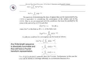
Example 2.17 Absolute
2.17 Absolute Summability
Summability for
for A
A S
Sudden
udden-
-Applied Exponential
Applied Exponential
<
<
=
=
=
∑ ω
∞
ω
−
ω
1
|
a
|
or
ae
|
for
e
a
X(e
is
sequence
this
of
transform
Fourier
The
n
u
a
x[n]
Consider
j
-
n
j
n
j
n
1
|
1
)
].
[
<
<
<
−
=
= ∑ ω
−
=
i.e.,
x[n];
of
ty
summabili
absolute
the
for
condition
the
is
1
|
a
|
conidtion
the
Clearly,
1
|
a
|
or
ae
|
for
ae
e
a
X(e
j
n
1
|
1
)
0
∞
<
−
=
= ∑
∞
=
ω
a
a
X(e
n
n
j
|
|
1
1
|
|
)
0](https://image.slidesharecdn.com/ch2discretetimesignalandsystems-230606064019-94a62f87/85/Ch2_Discrete-time-signal-and-systems-pdf-53-320.jpg)
![Discrete-Time Signal Processing, 2/E by Alan V. Oppenheim and Ronald W. Schafer
Chapter 2 Discrete
Chapter 2 Discrete-
-Time Signal and Systems
Time Signal and Systems
⎧ ≤
|
|
1
Example 2.18 Square
Example 2.18 Square-
-summability
summability for the ideal
for the ideal lowpass
lowpass filter
filter
⎩
⎨
⎧
π
≤
ω
≤
ω
ω
≤
ω
=
ω
|
|
,
0
|
|
,
1
)
e
(
H
c
c
j
lp
π
=
ω
π
= ω
ω
−
ω
ω
ω
−
ω
∫ ]
e
[
jn
2
1
d
e
2
1
]
n
[
h n
j
n
j
lp
c
c
c
c
Ideal lowpass requires infinite
Ideal lowpass requires infinite
points
points
∞
<
<
−∞
π
ω
=
−
π
= ω
−
ω
n
,
n
n
sin
)
e
e
(
jn
2
1 c
n
j
n
j c
c
In real cases, the filter lengths can not be infinite
In real cases, the filter lengths can not be infinite
θ
θ
−
ω
θ
−
ω
+
π
=
π
ω
= ∫
∑
ω
ω
ω
−
−
=
ω
d
2
/
)]
sin[(
]
2
/
)
)(
1
M
2
sin[(
2
1
e
n
n
sin
)
e
(
H
c
c
n
j
M
M
n
c
j
M
)]
[(](https://image.slidesharecdn.com/ch2discretetimesignalandsystems-230606064019-94a62f87/85/Ch2_Discrete-time-signal-and-systems-pdf-54-320.jpg)
![Discrete-Time Signal Processing, 2/E by Alan V. Oppenheim and Ronald W. Schafer
Chapter 2 Discrete
Chapter 2 Discrete-
-Time Signal and Systems
Time Signal and Systems
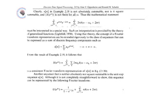
Example 2.19 Fourier Transform of a constant
Example 2.19 Fourier Transform of a constant
Consider x[n] =1 for all n. This sequence is neither absolutely summable nor
bl Th F i t f f th [ ] i th i di
square summable. The Fourier transform of the sequence x[n] is the periodic
impulse train
∑
∞
ω
π
+
ω
πδ
=
j
)
r
(
)
e
(
X 2
2
∑
−∞
=
r
)
(
)
(
Consider the inverse Fourier transform,
1
∫ ∑
∞
π
1
)
2
(
2
2
1
]
[ =
⋅
+
= ∫ ∑
−
−∞
=
ω
π
ω
πδ
π
ω
π
π
d
e
r
n
x n
j
r
Example 2.20 Fourier Transform of complex Exponential Sequences
Example 2.20 Fourier Transform of complex Exponential Sequences
∑
∞
−∞
=
ω
π
+
ω
−
ω
πδ
=
r
j
)
r
(
)
e
(
X 2
2 0
1 π ∞
∫
n
j
r
d
e
r
n
x 0
1
)
2
(
2
2
1
]
[ ω
π
π
ω
π
ω
ω
πδ
π
⋅
+
−
=
∞
−
−∞
=
∫ ∑
n
j
n
j
n
j
r
e
e
d
e
r 0
0
0 )
(
0 )
2
(
2
2
1 ω
ω
ω
ω
π
π
ω
π
ω
ω
πδ
π
=
⋅
⋅
+
−
= −
−
∞
−∞
=
∫ ∑](https://image.slidesharecdn.com/ch2discretetimesignalandsystems-230606064019-94a62f87/85/Ch2_Discrete-time-signal-and-systems-pdf-56-320.jpg)
![Discrete-Time Signal Processing, 2/E by Alan V. Oppenheim and Ronald W. Schafer
Discrete-Time Fourier Transform of Unit Step Function
1
1/2
1/2
= +
1/2
-1/2
1
1 1/2
}
)
2
(
{
2
1
,
)
2
(
2
}
1
{
2
1
]
[
2
1
]
[
1
r
π
ω
πδ
F
r
π
ω
πδ
F
n
Sqn
n
u
+
=
∴
+
=
+
=
∞
−
∞
∑
∑
Q
2
1
2
1
]}
[
{
,
0
,
1
0
,
1
]
[
2
0
1
e
α
e
α
n
Sqn
F
n
n
n
Sqn
n
n
ω
j
n
n
n
ω
j
n
r
r
+
−
=
∴
⎩
⎨
⎧
<
−
≥
=
∞
=
−
−
−∞
=
−
−
−∞
=
−∞
=
∑
∑
∑
∑
1
1
1
1
1
1
1
1
2
1
)
(
1
1
1
2
1
2
1
)
(
1
2
1
1
0
0
'
1
'
'
e
α
e
α
e
α
e
α
ω
j
ω
j
ω
j
n
n
ω
j
n
n
n
ω
j
n
⎞
⎛
−
+
⎟
⎟
⎠
⎞
⎜
⎜
⎝
⎛
−
−
=
+
⎟
⎠
⎞
⎜
⎝
⎛
−
=
−
−
−
−
∞
=
−
∞
=
−
−
∑
∑
1
1
1
1
1
2
1
2
1
1
1
2
1
1
2
1
α
e
α
α
e
α
e
α
α
e
e
ω
j
ω
j
ω
j
ω
j
ω
j
+
=
−
+
−
−
=
−
+
⎟
⎟
⎠
⎞
⎜
⎜
⎝
⎛
−
−
= −
−
−
−
)
(
1
1
2
1
1
1
2
1
)}
(
{
,
1
1
2
2
ω
πδ
e
e
t
u
F
then
α
for
e
α
e
α
ω
j
ω
j
ω
j
ω
j
+
−
+
−
=
⇒
=
−
+
−
=
−
−
−
−](https://image.slidesharecdn.com/ch2discretetimesignalandsystems-230606064019-94a62f87/85/Ch2_Discrete-time-signal-and-systems-pdf-58-320.jpg)
![Discrete-Time Signal Processing, 2/E by Alan V. Oppenheim and Ronald W. Schafer
Chapter 2 Discrete
Chapter 2 Discrete-
-Time Signal and Systems
Time Signal and Systems
Example 2.19 Fourier Transform of
Example 2.19 Fourier Transform of Complex Exponential Sequences
Complex Exponential Sequences
Consider a sequence x[n] whose Fourier transform is the periodic impulse train
∑
∞
ω
π
+
ω
−
ω
πδ
=
j
r
e
X )
2
(
2
)
( 0
−∞
=
r
Applying inverse Fourier transform, we have
( ) n
j
n
j
j
d
e
d
e
e
X
n
x
π
π
−
ω
π
π
−
ω
ω
ω
⋅
ω
−
ω
πδ
π
=
ω
⋅
π
=
∫
∫ 0
2
2
1
)
(
2
1
]
[
n
j 0
e ω
=](https://image.slidesharecdn.com/ch2discretetimesignalandsystems-230606064019-94a62f87/85/Ch2_Discrete-time-signal-and-systems-pdf-59-320.jpg)
![Discrete-Time Signal Processing, 2/E by Alan V. Oppenheim and Ronald W. Schafer
Chapter 2 Discrete
Chapter 2 Discrete-
-Time Signal and Systems
Time Signal and Systems
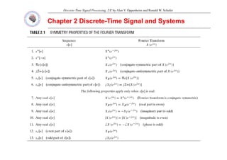
2.8 Symmetry Properties of The Fourier Transform
2.8 Symmetry Properties of The Fourier Transform
Definition
Definition
Definition
Definition
Conjugate
Conjugate-
-symmetric sequence:
symmetric sequence:
C j t
C j t ti t i
ti t i
]
n
[
x
])
n
[
*
x
]
n
[
x
(
]
n
[
x *
e
e −
=
−
+
=
2
1
]
[
])
[
*
]
[
(
]
[ *
1
]
n
[
x
]
n
[
x
]
n
[
x o
e +
=
Conjugate
Conjugate-
-antisymmetric sequence:
antisymmetric sequence: ]
n
[
x
])
n
[
*
x
]
n
[
x
(
]
n
[
x o
o −
−
=
−
−
=
2
Summation
Summation
Odd
Odd
Even sequence
Even sequence Odd sequence
Odd sequence
Definition
Definition
Conj gate
Conj gate s mmetric seq ence
s mmetric seq ence )
e
(
X
))
e
(
*
X
)
e
(
X
(
)
e
(
X j
*
j
j
j ω
−
ω
−
ω
ω
=
+
=
1
Conjugate
Conjugate-
-symmetric sequence:
symmetric sequence:
Conjugate
Conjugate-
-antisymmetric sequence:
antisymmetric sequence:
)
e
(
X
))
e
(
*
X
)
e
(
X
(
)
e
(
X e
e =
+
=
2
)
e
(
X
))
e
(
*
X
)
e
(
X
(
)
e
(
X j
*
o
j
j
j
o
ω
−
ω
−
ω
ω
−
=
−
=
2
1
Summation
Summation )
e
(
X
)
e
(
X
)
e
(
X j
o
j
e
j ω
ω
ω
+
=
Even spectrum
Even spectrum Odd spectrum
Odd spectrum](https://image.slidesharecdn.com/ch2discretetimesignalandsystems-230606064019-94a62f87/85/Ch2_Discrete-time-signal-and-systems-pdf-60-320.jpg)
![Discrete-Time Signal Processing, 2/E by Alan V. Oppenheim and Ronald W. Schafer
Chapter 2 Discrete
Chapter 2 Discrete-
-Time Signal and Systems
Time Signal and Systems
2.9 Fourier Transform Theorems
2.9 Fourier Transform Theorems
]}
n
[
x
{
F
)
e
(
X jω
=
)}
e
(
X
{
F
]
n
[
x
]}
n
[
x
{
F
)
e
(
X
F
jω
−
= 1
2.9.1 Linearity of the Fourier Transform
2.9.1 Linearity of the Fourier Transform
)
e
(
X
]
n
[
x j
F
ω
↔
)
e
(
X
]
n
[
x
F
j
F
ω
↔ 1
1
)
e
(
X
]
n
[
x j
F
ω
↔ 2
2
)
(
bX
)
(
X
]
[
b
]
[ j
j
F
ω
ω
)
e
(
bX
)
e
(
aX
]
n
[
bx
]
n
[
ax j
j ω
ω
+
↔
+ 2
1
2
1](https://image.slidesharecdn.com/ch2discretetimesignalandsystems-230606064019-94a62f87/85/Ch2_Discrete-time-signal-and-systems-pdf-63-320.jpg)
![Discrete-Time Signal Processing, 2/E by Alan V. Oppenheim and Ronald W. Schafer
Chapter 2 Discrete
Chapter 2 Discrete-
-Time Signal and Systems
Time Signal and Systems
2.9.2 Time Shifting and Frequency Shifting
2.9.2 Time Shifting and Frequency Shifting
F
)
e
(
X
]
n
[
x j
F
ω
↔
Time shifting
Time shifting )
e
(
X
e
]
n
n
[
x j
n
j
F
d ω
ω
−
⋅
↔
−
Time shifting
Time shifting )
e
(
X
e
]
n
n
[
x d ↔
Frequency shifting
Frequency shifting )
e
(
X
]
n
[
x
e )
(
j
F
n
j 0
0 ω
−
ω
ω
↔
2.9.3 Time Reversal
2.9.3 Time Reversal
j
F
ω
)
e
(
X
]
n
[
x jω
↔
X[n] is time reversed
X[n] is time reversed )
e
(
X
]
n
[
x j
F
ω
−
↔
− )
(
]
[
X[n] is real and time reversed
X[n] is real and time reversed )
e
(
X
]
n
[
x j
*
F
ω
↔
−
Conjugate-symmetric](https://image.slidesharecdn.com/ch2discretetimesignalandsystems-230606064019-94a62f87/85/Ch2_Discrete-time-signal-and-systems-pdf-64-320.jpg)
![Discrete-Time Signal Processing, 2/E by Alan V. Oppenheim and Ronald W. Schafer
Chapter 2 Discrete
Chapter 2 Discrete-
-Time Signal and Systems
Time Signal and Systems
2.9.4 Differentiation in Frequency
2.9.4 Differentiation in Frequency
F
)
e
(
X
]
n
[
x j
F
ω
↔
ω
)
(
dX j
F
ω
↔
ω
d
)
e
(
dX
j
]
n
[
nx
j
F
then
2.9.5 Parseval’s Theorem
2.9.5 Parseval’s Theorem
)
e
(
X
]
n
[
x j
F
ω
↔ )
e
(
X
]
n
[
x ↔
∫
∑
π
ω
∞
ω
=
= d
|
)
e
(
X
|
|
]
n
[
x
|
E j 2
2 1
then
∫
∑ π
−
−∞
= π
|
)
(
|
|
]
[
|
n 2](https://image.slidesharecdn.com/ch2discretetimesignalandsystems-230606064019-94a62f87/85/Ch2_Discrete-time-signal-and-systems-pdf-65-320.jpg)
![Discrete-Time Signal Processing, 2/E by Alan V. Oppenheim and Ronald W. Schafer
Chapter 2 Discrete
Chapter 2 Discrete-
-Time Signal and Systems
Time Signal and Systems
2.9.6 The Convolution Theorem
2.9.6 The Convolution Theorem
F
)
e
(
X
]
n
[
x j
F
ω
↔
)
(
H
]
[
h j
F
ω
↔ )
e
(
H
]
n
[
h jω
↔
∑
∞
=
−
= ]
n
[
h
*
]
n
[
x
]
k
n
[
h
]
k
[
x
]
n
[
y ∑
−∞
=
n
]
[
]
[
]
[
]
[
]
[
y
)
e
(
H
)
e
(
X
)
e
(
Y j
j
j ω
ω
ω
=
Then
Then
∑
∑
∑
∞
ω
−
∞
∞
ω
−
ω n
j
n
j
j
e
]
k
n
[
h
]
k
[
x
e
]
n
[
y
)
e
(
Y
)
e
(
H
)
e
(
X
)
e
(
Y j
j
j
=
Then
Then
∑ ∑
∑
∑
∑
∞ ∞
−∞
=
−∞
=
−∞
=
−
=
=
j
j
j
k
j
k
j
n
n
j
j
e
]
k
n
[
h
]
k
[
x
e
]
n
[
y
)
e
(
Y
∑ ∑
−∞
=
ω
ω
ω
−
−∞
=
ω
−
=
⋅
=
m
j
j
m
j
k
k
j
)
e
(
H
)
e
(
X
e
)
e
]
k
[
x
](
m
[
h](https://image.slidesharecdn.com/ch2discretetimesignalandsystems-230606064019-94a62f87/85/Ch2_Discrete-time-signal-and-systems-pdf-66-320.jpg)
![Discrete-Time Signal Processing, 2/E by Alan V. Oppenheim and Ronald W. Schafer
Chapter 2 Discrete
Chapter 2 Discrete-
-Time Signal and Systems
Time Signal and Systems
)
(
X
]
[ j
F
ω
↔
Consider ideal delay system
Consider ideal delay system
)
e
(
X
]
n
[
x jω
↔
d
n
j
F
d e
]
n
n
[ ω
−
↔
−
δ d ]
[
d
n
j
j
j
F
d e
)
e
(
X
)
e
(
Y
]
n
n
[
*
]
n
[
x
]
n
[
y ω
−
ω
ω
=
↔
−
δ
=](https://image.slidesharecdn.com/ch2discretetimesignalandsystems-230606064019-94a62f87/85/Ch2_Discrete-time-signal-and-systems-pdf-67-320.jpg)
![Discrete-Time Signal Processing, 2/E by Alan V. Oppenheim and Ronald W. Schafer
Chapter 2 Discrete
Chapter 2 Discrete-
-Time Signal and Systems
Time Signal and Systems
2.9.7 The Modulation or Windowing Theorem
2.9.7 The Modulation or Windowing Theorem
)
(
X
]
[ j
F ω
)
e
(
W
]
n
[
W
)
e
(
X
]
n
[
x
j
F
j
F
ω
ω
⎯→
←
⎯→
←
then ]
n
[
w
]
n
[
x
]
n
[
y =
∫
π
θ
θ )
(
j
j
1
∫
π
π
−
θ
−
ω
θ
θ
π
d
)
e
(
W
)
e
(
X )
(
j
j
2
1
C id n
j
]
[
]
[
]}
[
{
F ω
−
∞
∑
Consider n
j
e
]
n
[
w
]
n
[
x
]}
n
[
y
{
F ω
∞
−
∑
=
When ω =0,
0
0 =
ω
ω
−
∞
∞
−
=
ω = ∑ |
e
]
n
[
x
]
n
[
x
|
]}
n
[
y
{
F n
j
*
0
2
1
=
ω
ω
−
θ
π
π
−
θ
θ
π
= ∫ |
d
)
e
(
X
)
e
(
X )
(
j
*
j
Parseval’s Theorem](https://image.slidesharecdn.com/ch2discretetimesignalandsystems-230606064019-94a62f87/85/Ch2_Discrete-time-signal-and-systems-pdf-68-320.jpg)
![Discrete-Time Signal Processing, 2/E by Alan V. Oppenheim and Ronald W. Schafer
]
[
]
[
]
[
)
1
( n
n
n
n
u
a
n
u
na
n
u
a
n
Check +
=
+
1
1
1
1
1
1
ω
j
ω
j
ω
j
DTFT
ae
ae
ae
ω
d
d
j
−
−
−
−
+
⎥
⎦
⎤
⎢
⎣
⎡
−
⎯
⎯ →
⎯
( ) ( )2
2
1
1
1
1
1 ω
j
ω
j
ω
j
ae
ae
ae
ae
−
−
−
−
=
−
+
−
=](https://image.slidesharecdn.com/ch2discretetimesignalandsystems-230606064019-94a62f87/85/Ch2_Discrete-time-signal-and-systems-pdf-69-320.jpg)
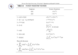
![Discrete-Time Signal Processing, 2/E by Alan V. Oppenheim and Ronald W. Schafer
Chapter 2 Discrete
Chapter 2 Discrete-
-Time Signal and Systems
Time Signal and Systems
Example
Example 2.22
2.22
ω
−
ω
−
=
= ,
1
1
)
]
[
n
j
j
1
n
1
e
(e
X
transform
Fourier
its
with
n
u
a
[n]
x
For
−
= ].
5
[
]
[ n
A
n
u
a
n
x
of
transform
Fourier
the
find
please
( ) ω
−
ω
⋅
⎯→
⎯
− 0]
[
:
0
n
j
j
F
e
e
X
n
n
x
Answer
Q
{ } −
ω
−
−
=
⋅
=
∴
=
−
=
−
=
5
5
2
2
1
5
]}
[
{
1
]
[
].
[
]
5
[
]
5
[
]
[
j
j
n
5
-
n
x
a
F
e
n
x
F
n
x
n
x
n
u
a
n
x
a
and
{ }
{ } { } ω
−
ω
−
⋅
=
=
⇒
−
5
5
2
5
2
]
[
]
[
]}
[
{
1
]
[
j
j
j
e
a
n
x
F
a
n
x
F
a
{ } { } ω
−
−
2
1
]
[
]
[
j
a](https://image.slidesharecdn.com/ch2discretetimesignalandsystems-230606064019-94a62f87/85/Ch2_Discrete-time-signal-and-systems-pdf-71-320.jpg)
![Discrete-Time Signal Processing, 2/E by Alan V. Oppenheim and Ronald W. Schafer
Chapter 2 Discrete
Chapter 2 Discrete-
-Time Signal and Systems
Time Signal and Systems
Example
Example 2.23
2.23
f
T f
F i
i
th
fi d
Pl
( ) )
1
)(
1
(
1
be
ae
e
X
of
Transform
Fourier
inverse
the
find
Please
j
j
j
−
−
=
ω
−
ω
−
ω
:
)
1
)(
1
(
Answer
be
ae
( ) 1
)
/(
1
)
/(
)
1
)(
1
(
1
be
b
a
b
ae
b
a
a
be
ae
e
X
j
j
j
j
j
⎞
⎛
⎞
⎛
−
−
−
−
−
=
−
−
=
ω
−
ω
−
ω
−
ω
−
ω
]
[
]
[
]
[
1
n
u
b
b
a
b
n
u
a
b
a
a
n
x n
n
F
⎟
⎠
⎞
⎜
⎝
⎛
−
−
⎟
⎠
⎞
⎜
⎝
⎛
−
=
⎯
⎯ →
⎯
−](https://image.slidesharecdn.com/ch2discretetimesignalandsystems-230606064019-94a62f87/85/Ch2_Discrete-time-signal-and-systems-pdf-72-320.jpg)
![Discrete-Time Signal Processing, 2/E by Alan V. Oppenheim and Ronald W. Schafer
Chapter 2 Discrete
Chapter 2 Discrete-
-Time Signal and Systems
Time Signal and Systems
Example
Example 2.24
2.24
is
phase
linear
with
filter
highpass
a
of
response
frequency
The
0
|
|
)
(
c
c
n
j
j
|
|
,
,
e
e
H
p
f
g p
f
p
f q y
d
⎪
⎩
⎪
⎨
⎧
ω
<
ω
π
<
ω
<
ω
=
ω
−
ω
( ) )
(
)
(
1
)
( j
lp
n
j
n
j
j
lp
n
j
j
c
e
H
e
e
e
H
e
e
H
as
expressed
be
can
response
frequency
This
.
understood
is
2
of
period
a
where
d
d
d −
=
−
=
π
⎩
ω
ω
−
ω
−
ω
ω
−
ω
( )
{ }
)
(
sin
,
sin
)
(
d
j
c
j
lp
1
-
p
p
n
n
n
n
e
H
F
Since
ω
π
ω
=
ω
)
(
)
(
sin
]
[
)
(
d
d
c
d
j
n
n
n
n
n
n
e
H
−
π
−
ω
−
−
δ
=
∴ ω](https://image.slidesharecdn.com/ch2discretetimesignalandsystems-230606064019-94a62f87/85/Ch2_Discrete-time-signal-and-systems-pdf-73-320.jpg)


![Digital Signal Processing[ECEG-3171]-Ch1_L03](https://cdn.slidesharecdn.com/ss_thumbnails/dspl3-180427094423-thumbnail.jpg?width=640&height=640&fit=bounds)