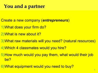
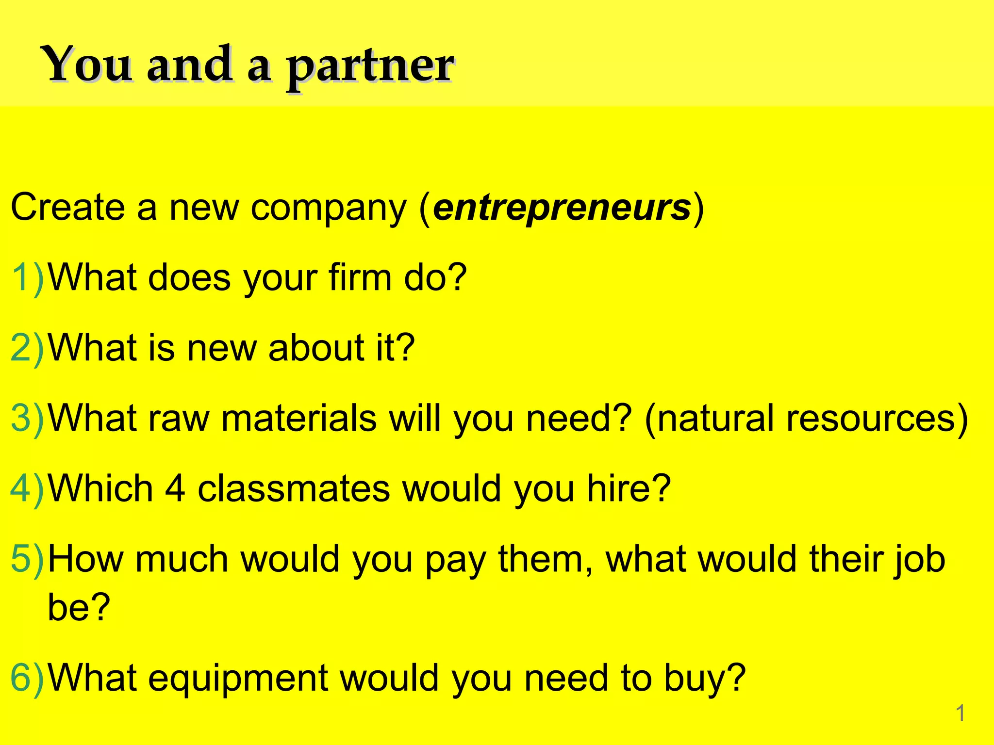
You and a partner
Create a new company (entrepreneurs)
1)What does your firm do?
2)What is new about it?
3)What raw materials will you need? (natural resources)
4)Which 4 classmates would you hire?
5)How much would you pay them, what would their job
be?
6)What equipment would you need to buy?

1
Factors of Production and Factor Markets

 Factors of production: the
inputs used to produce goods
and services.
 Labor
 Land

 Capital: the equipment and
structures used
to produce goods and services.

 Prices and quantities of these
inputs are determined by
supply & demand in factor
markets.
Derived Demand

 Markets for the factors of production are like
markets for goods & services, except:
 Demand for a factor of production is a derived
demand – derived from a firm’s decision to supply
a good in another market.
 How much will I make from this?

THE MARKETS FOR THE FACTORS OF PRODUCTION

3
Two Assumptions
1. We assume all markets are

competitive.
The typical firm is a price taker
 in the market for the product it
produces
 in the labor market
2. We assume that firms care only

about maximizing profits.
 Each firm’s supply of output
and demand for inputs are
derived from this goal.
Our Example: Farmer Jack
 Farmer Jack sells wheat in a
perfectly competitive market.
 He hires workers in a perfectly
competitive labor market.
 When deciding how many
workers to hire, Farmer Jack
maximizes profits by
thinking at the margin:
 If the benefit from hiring
another worker exceeds the
cost, Jack will hire that worker.
Our Example: Farmer Jack
 Cost of hiring another worker:
the wage – the price of labor
 Benefit of hiring another worker:
Jack can produce more wheat
to sell,increasing his revenue.
 The size of this benefit depends
on Jack’s production function:
the relationship between the
quantity of inputs used to make a
good and the quantity of output of
that good.
Farmer Jack’s Production Function
Q

(bushels
(no. of
of wheat
workers) per week)

3,000

Quantity of output

L

2,500

0

0

1

1000

2

1800

3

2400

500

4

2800

0

5

3000

2,000
1,500
1,000

0

1

2

3

4

5

No. of workers

THE MARKETS FOR THE FACTORS OF PRODUCTION

7
Marginal Product of Labor (MPL)
 Marginal product of labor: the increase in the
amount of output from an additional unit of labor

∆Q
MPL =
∆L

where
∆Q = change in output
∆L = change in labor
THE MARKETS FOR THE FACTORS OF PRODUCTION
The Marginal Revenue Product
 Problem:
 Cost of hiring another worker
(wage) is measured in dollars
 Benefit of hiring another worker
(MPL) is measured in units of
output
 Solution: convert MPL to dollars
 Value of the marginal product:
the marginal product of an input
times the price of the output
VMPL = value of the marginal
product of labor (marginal revenue
= P x MPL
Same concept, different names
Value of Marginal Product = Mankiw
Marginal Revenue Labor Product = College Board
ACTIVE LEARNING

1

Computing MPL and MRPL (VMPL)
P = $5/bushel.
Find MPL
and MRPL,
fill them in the
blank spaces
of the table.
Then graph
a curve with
VMPL on the
vertical axis,
L on horiz axis.

L
Q
(no. of
(bushels
workers) of wheat)
0

1000

2

1800

3

2400

4

2800

5

MRPL

0

1

MPL

3000
14
ACTIVE LEARNING

Answers
Farmer Jack’s
production
function
exhibits
diminishing
marginal
product:
MPL falls as
L increases.
This property is
very common.

1

L
Q
MPL = MRPL=
(no. of
(bushels
workers) of wheat) ∆Q/∆L P x MPL
0

0

1

1000

2

1800

3

2400

4

2800

5

3000

1000

$5,000

800

4,000

600

3,000

400

2,000

200

1,000

15
ACTIVE LEARNING

Answers
Farmer Jack’s
VMPL curve is
downward
sloping
due to
diminishing
marginal
product.

1

The VMPL curve

$6,000
5,000
4,000
3,000
2,000
1,000
0

0

1
2
3
4
L (number of workers)

5
16
Farmer Jack’s Labor Demand
Suppose wage
W = $2500/week.
How many
workers should
Jack hire?

$6,000

The VMPL curve

5,000
4,000

3,000
Answer: L = 3
$2,50
At any larger L,
02,000
can increase profit
by hiring one
1,000
fewer worker.
At any smaller L,
0
0
can increase profit
by hiring another
worker.

1
2
3
4
L (number of workers)

5
17
VMPL and Labor Demand
For any competitive,
profit-maximizing firm:
 To maximize profits,
hire workers up to
the point where
VMPL = W.

W

W1

 The VMPL curve is
the labor demand
curve.

VMPL
L1

THE MARKETS FOR THE FACTORS OF PRODUCTION

L

18
Shifts in Labor Demand
Labor demand curve
= VMPL curve.

W

VMPL = P x MPL
Anything that
increases P or
MPL at each L
will increase
VMPL and shift
labor demand curve
upward.
THE MARKETS FOR THE FACTORS OF PRODUCTION

D2
D1
L

19
Things that Shift the Labor Demand Curve
 Changes in the output price, P
 Technological change (affects MPL)
 The supply of other factors (affects MPL)
 Example:
If firm gets more equipment (capital),
then workers will be more productive;
MPL and VMPL rise, labor demand shifts
upward.

THE MARKETS FOR THE FACTORS OF PRODUCTION

20
The Connection Between Input Demand
& Output Supply
 Recall: Marginal Cost (MC)
= cost of producing an additional unit of output
= ∆TC/∆Q, where TC = total cost
 Suppose W = $2500, MPL = 500 bushels
 If Farmer Jack hires another worker,
∆TC = $2500, ∆Q = 500 bushels
MC = $2500/500 = $5 per bushel
 In general:

MC = W/MPL

THE MARKETS FOR THE FACTORS OF PRODUCTION

21
The Connection Between Input Demand
& Output Supply
 In general:

MC = W/MPL

 Notice:
 To produce additional output, hire more labor.
 As L rises, MPL falls…
 causing W/MPL to rise…
 causing MC to rise.
 Hence, diminishing marginal product and
increasing marginal cost are two sides
of the same coin.
THE MARKETS FOR THE FACTORS OF PRODUCTION

22
The Connection Between Input Demand
& Output Supply
 The competitive firm’s rule for demanding labor:
P x MPL = W
 Divide both sides by MPL:
P = W/MPL
 Substitute MC = W/MPL from previous slide:
P = MC
 This is the competitive firm’s rule for supplying
output.
 Hence, input demand and output supply are two
sides of the same coin.
THE MARKETS FOR THE FACTORS OF PRODUCTION

23
Labor Supply
 Trade-off between work
and leisure:
The more time you
spend working,
the less time you have
for leisure.
 The opportunity cost of
leisure is the wage.

THE MARKETS FOR THE FACTORS OF PRODUCTION

24
The Labor Supply Curve
An increase in W
is an increase in the
opp. cost of leisure.
People respond by
taking less leisure
and by working more.

W
S1
W2
W1

L1 L2
THE MARKETS FOR THE FACTORS OF PRODUCTION

L

25
Things that Shift the Labor Supply Curve
 Changes in tastes
or attitudes
regarding the
labor-leisure
trade-off
 Opportunities for
workers in other
labor markets
 Immigration

THE MARKETS FOR THE FACTORS OF PRODUCTION

26
Equilibrium in the Labor Market
The wage adjusts to
balance supply and
demand for labor.

W
S

The wage always equals
VMPL.
W1

D
L1
THE MARKETS FOR THE FACTORS OF PRODUCTION

L

27
Mankiw homework
 Pages 394-395
 #1, 3, 4, 5, 6
ACTIVE LEARNING

2

Changes in labor-market equilibrium
In each of the following scenarios, use a diagram of
the market for (domestic) auto workers to find the
effects on their wage and employment.
A. Baby Boomers who worked in the auto industry
retire.
B. Car buyers’ preferences shift toward imported
autos.
C. Technological progress boosts productivity
in the auto manufacturing industry.
29
2

ACTIVE LEARNING

Answers to A
The retirement of
Baby Boomer auto
workers shifts
supply leftward.
W rises, L falls.

W

The market for
The market for
autoworkers
autoworkers
S2
S1

W2
W1

D1
L2 L1

L
30
2

ACTIVE LEARNING

Answers to B
A fall in the demand
for U.S. autos
reduces P.
At each L,
VMPL falls.
Labor demand
curve shifts down.

W

The market for
The market for
autoworkers
autoworkers
S1

W1
W2

W and L both fall.

D2
L2 L1

D1
L
31
2

ACTIVE LEARNING

Answers to C
At each L,
MPL rises due to
tech. progress.
VMPL rises and
labor demand curve
shifts upward.

W

The market for
The market for
autoworkers
autoworkers
S1

W2
W1
D2

W and L increase.
D1
L1 L2

L
32
Linkages Among the Factors of Production
 In most cases, factors of
production are used together in a
way that makes each factor’s
productivity dependent on the
quantities of the other factors.
 Example: an increase in the
quantity of capital
 The marginal product and rental
price of capital fall.
 Having more capital makes
workers more productive, MPL
and W rise.
1995 FRQ, with 1 partner
#3, #4 EC 6 -7

Factor markets

  • 1.
    You and apartner Create a new company (entrepreneurs) 1)What does your firm do? 2)What is new about it? 3)What raw materials will you need? (natural resources) 4)Which 4 classmates would you hire? 5)How much would you pay them, what would their job be? 6)What equipment would you need to buy? 1
  • 2.
    Factors of Productionand Factor Markets  Factors of production: the inputs used to produce goods and services.  Labor  Land  Capital: the equipment and structures used to produce goods and services.  Prices and quantities of these inputs are determined by supply & demand in factor markets.
  • 3.
    Derived Demand  Marketsfor the factors of production are like markets for goods & services, except:  Demand for a factor of production is a derived demand – derived from a firm’s decision to supply a good in another market.  How much will I make from this? THE MARKETS FOR THE FACTORS OF PRODUCTION 3
  • 4.
    Two Assumptions 1. Weassume all markets are competitive. The typical firm is a price taker  in the market for the product it produces  in the labor market 2. We assume that firms care only about maximizing profits.  Each firm’s supply of output and demand for inputs are derived from this goal.
  • 5.
    Our Example: FarmerJack  Farmer Jack sells wheat in a perfectly competitive market.  He hires workers in a perfectly competitive labor market.  When deciding how many workers to hire, Farmer Jack maximizes profits by thinking at the margin:  If the benefit from hiring another worker exceeds the cost, Jack will hire that worker.
  • 6.
    Our Example: FarmerJack  Cost of hiring another worker: the wage – the price of labor  Benefit of hiring another worker: Jack can produce more wheat to sell,increasing his revenue.  The size of this benefit depends on Jack’s production function: the relationship between the quantity of inputs used to make a good and the quantity of output of that good.
  • 7.
    Farmer Jack’s ProductionFunction Q (bushels (no. of of wheat workers) per week) 3,000 Quantity of output L 2,500 0 0 1 1000 2 1800 3 2400 500 4 2800 0 5 3000 2,000 1,500 1,000 0 1 2 3 4 5 No. of workers THE MARKETS FOR THE FACTORS OF PRODUCTION 7
  • 8.
    Marginal Product ofLabor (MPL)  Marginal product of labor: the increase in the amount of output from an additional unit of labor ∆Q MPL = ∆L where ∆Q = change in output ∆L = change in labor
  • 9.
    THE MARKETS FORTHE FACTORS OF PRODUCTION
  • 10.
    THE MARKETS FORTHE FACTORS OF PRODUCTION
  • 11.
    THE MARKETS FORTHE FACTORS OF PRODUCTION
  • 12.
    The Marginal RevenueProduct  Problem:  Cost of hiring another worker (wage) is measured in dollars  Benefit of hiring another worker (MPL) is measured in units of output  Solution: convert MPL to dollars  Value of the marginal product: the marginal product of an input times the price of the output VMPL = value of the marginal product of labor (marginal revenue = P x MPL
  • 13.
    Same concept, differentnames Value of Marginal Product = Mankiw Marginal Revenue Labor Product = College Board
  • 14.
    ACTIVE LEARNING 1 Computing MPLand MRPL (VMPL) P = $5/bushel. Find MPL and MRPL, fill them in the blank spaces of the table. Then graph a curve with VMPL on the vertical axis, L on horiz axis. L Q (no. of (bushels workers) of wheat) 0 1000 2 1800 3 2400 4 2800 5 MRPL 0 1 MPL 3000 14
  • 15.
    ACTIVE LEARNING Answers Farmer Jack’s production function exhibits diminishing marginal product: MPLfalls as L increases. This property is very common. 1 L Q MPL = MRPL= (no. of (bushels workers) of wheat) ∆Q/∆L P x MPL 0 0 1 1000 2 1800 3 2400 4 2800 5 3000 1000 $5,000 800 4,000 600 3,000 400 2,000 200 1,000 15
  • 16.
    ACTIVE LEARNING Answers Farmer Jack’s VMPLcurve is downward sloping due to diminishing marginal product. 1 The VMPL curve $6,000 5,000 4,000 3,000 2,000 1,000 0 0 1 2 3 4 L (number of workers) 5 16
  • 17.
    Farmer Jack’s LaborDemand Suppose wage W = $2500/week. How many workers should Jack hire? $6,000 The VMPL curve 5,000 4,000 3,000 Answer: L = 3 $2,50 At any larger L, 02,000 can increase profit by hiring one 1,000 fewer worker. At any smaller L, 0 0 can increase profit by hiring another worker. 1 2 3 4 L (number of workers) 5 17
  • 18.
    VMPL and LaborDemand For any competitive, profit-maximizing firm:  To maximize profits, hire workers up to the point where VMPL = W. W W1  The VMPL curve is the labor demand curve. VMPL L1 THE MARKETS FOR THE FACTORS OF PRODUCTION L 18
  • 19.
    Shifts in LaborDemand Labor demand curve = VMPL curve. W VMPL = P x MPL Anything that increases P or MPL at each L will increase VMPL and shift labor demand curve upward. THE MARKETS FOR THE FACTORS OF PRODUCTION D2 D1 L 19
  • 20.
    Things that Shiftthe Labor Demand Curve  Changes in the output price, P  Technological change (affects MPL)  The supply of other factors (affects MPL)  Example: If firm gets more equipment (capital), then workers will be more productive; MPL and VMPL rise, labor demand shifts upward. THE MARKETS FOR THE FACTORS OF PRODUCTION 20
  • 21.
    The Connection BetweenInput Demand & Output Supply  Recall: Marginal Cost (MC) = cost of producing an additional unit of output = ∆TC/∆Q, where TC = total cost  Suppose W = $2500, MPL = 500 bushels  If Farmer Jack hires another worker, ∆TC = $2500, ∆Q = 500 bushels MC = $2500/500 = $5 per bushel  In general: MC = W/MPL THE MARKETS FOR THE FACTORS OF PRODUCTION 21
  • 22.
    The Connection BetweenInput Demand & Output Supply  In general: MC = W/MPL  Notice:  To produce additional output, hire more labor.  As L rises, MPL falls…  causing W/MPL to rise…  causing MC to rise.  Hence, diminishing marginal product and increasing marginal cost are two sides of the same coin. THE MARKETS FOR THE FACTORS OF PRODUCTION 22
  • 23.
    The Connection BetweenInput Demand & Output Supply  The competitive firm’s rule for demanding labor: P x MPL = W  Divide both sides by MPL: P = W/MPL  Substitute MC = W/MPL from previous slide: P = MC  This is the competitive firm’s rule for supplying output.  Hence, input demand and output supply are two sides of the same coin. THE MARKETS FOR THE FACTORS OF PRODUCTION 23
  • 24.
    Labor Supply  Trade-offbetween work and leisure: The more time you spend working, the less time you have for leisure.  The opportunity cost of leisure is the wage. THE MARKETS FOR THE FACTORS OF PRODUCTION 24
  • 25.
    The Labor SupplyCurve An increase in W is an increase in the opp. cost of leisure. People respond by taking less leisure and by working more. W S1 W2 W1 L1 L2 THE MARKETS FOR THE FACTORS OF PRODUCTION L 25
  • 26.
    Things that Shiftthe Labor Supply Curve  Changes in tastes or attitudes regarding the labor-leisure trade-off  Opportunities for workers in other labor markets  Immigration THE MARKETS FOR THE FACTORS OF PRODUCTION 26
  • 27.
    Equilibrium in theLabor Market The wage adjusts to balance supply and demand for labor. W S The wage always equals VMPL. W1 D L1 THE MARKETS FOR THE FACTORS OF PRODUCTION L 27
  • 28.
    Mankiw homework  Pages394-395  #1, 3, 4, 5, 6
  • 29.
    ACTIVE LEARNING 2 Changes inlabor-market equilibrium In each of the following scenarios, use a diagram of the market for (domestic) auto workers to find the effects on their wage and employment. A. Baby Boomers who worked in the auto industry retire. B. Car buyers’ preferences shift toward imported autos. C. Technological progress boosts productivity in the auto manufacturing industry. 29
  • 30.
    2 ACTIVE LEARNING Answers toA The retirement of Baby Boomer auto workers shifts supply leftward. W rises, L falls. W The market for The market for autoworkers autoworkers S2 S1 W2 W1 D1 L2 L1 L 30
  • 31.
    2 ACTIVE LEARNING Answers toB A fall in the demand for U.S. autos reduces P. At each L, VMPL falls. Labor demand curve shifts down. W The market for The market for autoworkers autoworkers S1 W1 W2 W and L both fall. D2 L2 L1 D1 L 31
  • 32.
    2 ACTIVE LEARNING Answers toC At each L, MPL rises due to tech. progress. VMPL rises and labor demand curve shifts upward. W The market for The market for autoworkers autoworkers S1 W2 W1 D2 W and L increase. D1 L1 L2 L 32
  • 33.
    Linkages Among theFactors of Production  In most cases, factors of production are used together in a way that makes each factor’s productivity dependent on the quantities of the other factors.  Example: an increase in the quantity of capital  The marginal product and rental price of capital fall.  Having more capital makes workers more productive, MPL and W rise.
  • 40.
    1995 FRQ, with1 partner #3, #4 EC 6 -7

Editor's Notes

  • #6 We used this example in Chapter 13 to introduce the following concepts: production function marginal product of labor diminishing marginal product Here, we briefly review these concepts and then use them to derive Farmer Jack’s demand for labor.
  • #15 This exercise should not be difficult. But students are more likely to remember how to compute MPL and VMPL if we make them do it instead of just showing them the results. And students have computed lots of marginal things from preceding chapters, so they should be able to do this exercise using only the definitions of MPL and VMPL from the preceding slides.
  • #17 Some students may not offset the points between the L values, as shown here and in the table on the preceding slide. For our purposes, that’s okay. What matters is they see that VMPL is a downward-sloping curve. They will get the rest from the following slides.
  • #18 A student may wonder why we are measuring the wage in dollars per week rather than dollars per hour. If a student asks this question, before giving the answer, see if another student can explain the answer. The answer is: our task here is to compare the cost and benefit of hiring an extra worker. The benefit, P x MPL, is extra revenue per week from having one more workers (recall, the production function and hence MPL are measured in units per week). So we must compare that to the cost per week of having one more worker. The logic behind the answer L = 3 is the same marginal analysis that students have seen in many other contexts in previous chapters. At any L smaller than L = 3, can increase profit by hiring another worker. For example, suppose Jack has 2 workers. At L = 2, VMPL > W. In other words, the increase in revenue from hiring one more worker exceeds the increase in cost (the wage). So, hiring one more worker would increase profit. At any L larger than L = 3, can increase profit by hiring one fewer worker. For example, suppose Jack has 4 workers. At L = 4, VMPL < W. In other words, the revenue from the 4th worker is less than the cost of that worker, so Jack can increase profit by hiring one fewer worker.
  • #21 The example in the third point implies that the firm sees factor inputs as complements, not substitutes. While this is true in many cases, one can also think of examples in which the firm would see inputs as substitutes. For example, industrial robots have displaced some workers in the auto industry. Though, they have increased demand for other kinds of workers in that industry.
  • #22 This and the next two slides cover material from the FYI box entitled “Input Demand and Output Supply: Two Sides of the Same Coin.” This slide establishes the relationship between marginal cost and marginal product.
  • #23 This slide shows the connection between diminishing marginal product and increasing marginal cost.
  • #24 This slide shows that when a competitive firm hires labor to the point where W = VMPL, it is also producing output up to the point where P = MC. Hence, input demand and output supply are two sides of the same coin.
  • #26 At this point, the book briefly discusses the income and substitution effects. (The discussion is intuitive, and the actual terms “income and substitution effects” appear only parenthetically.) The book concedes the possibility that the labor supply curve might bend backward if the income effect exceeds the substitution effect, but states that we will ignore this possibility for now and assume the labor supply curve is positively sloped.
  • #27 Regarding the first point: The textbook notes that a change in attitudes about female labor force participation over the past 50 years has dramatically shifted the labor supply curve rightward.
  • #30 Again, these exercises should not be difficult, but students learn more if they do the exercises themselves. The exercise in Part C segues nicely into the case study on productivity and wages that follows.
  • #31 This scenario, in fact, will occur over the coming 10-15 years.