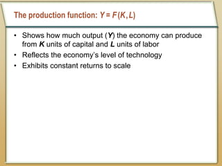
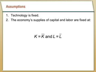
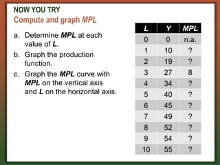
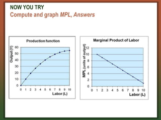
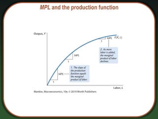
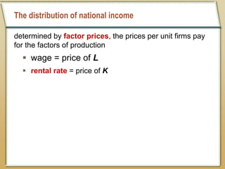
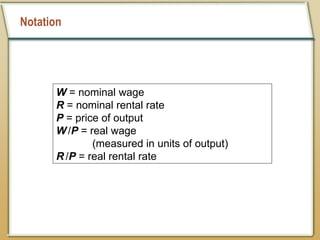
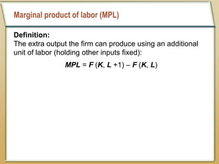
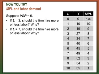
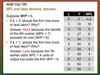
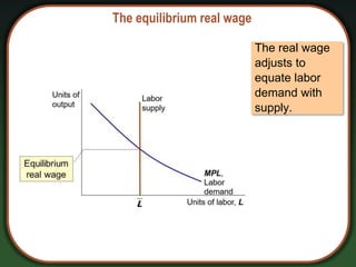
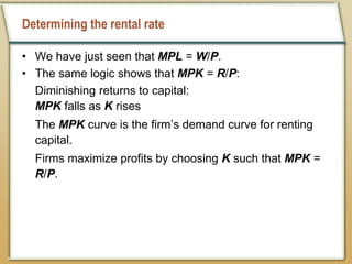
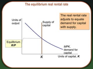
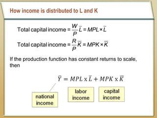
This document provides an overview of key concepts in macroeconomics including: - National income is determined by the production function based on the fixed supplies of capital and labor. - Factor prices like wages and rental rates are determined by supply and demand in factor markets and will equal the marginal product of each input. - Total income is distributed to capital and labor based on their marginal products. 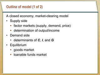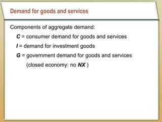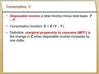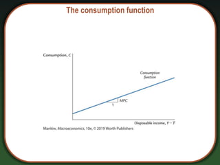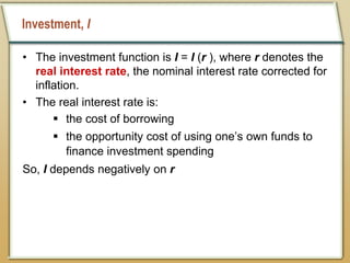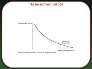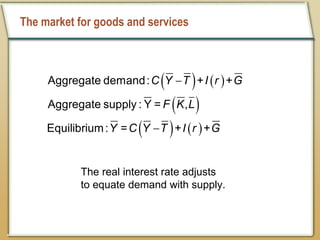- Aggregate demand is determined by consumption, investment, and government spending functions. 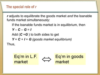- Equilibrium in the goods market occurs when aggregate demand equals supply as determined by the production function. 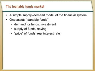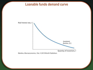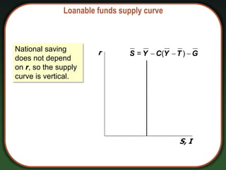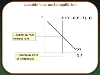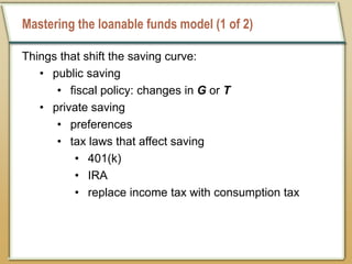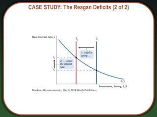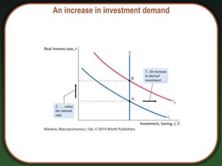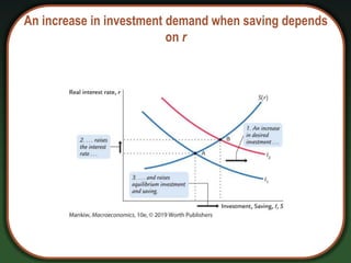- The loanable funds market equilibrates through adjustments in the real interest rate to equalize saving and investment

1. Presentation Slides
National Income:
Where it Comes
From and Where It
Goes
Macroeconomics
N. Gregory Mankiw
© 2019 Worth Publishers, all rights reserved

2. CHAPTER 3 National Income
CHAPTER 3 National Income
IN THIS CHAPTER, YOU WILL LEARN:
What determines the
economy’s total output/income
How the prices of the factors
of production are determined
How total income is distributed
What determines the demand
for goods and services
How equilibrium in the goods
market is achieved

3. Outline of model (1 of 2)
A closed economy, market-clearing model
• Supply side
 factor markets (supply, demand, price)
 determination of output/income
• Demand side
 determinants of C, I, and G
• Equilibrium
 goods market
 loanable funds market

4. Factors of production
K = capital:
tools, machines, and structures used in production
L = labor:
the physical and mental efforts of workers

5. The production function: Y = F(K,L)
• Shows how much output (Y) the economy can produce
from K units of capital and L units of labor
• Reflects the economy’s level of technology
• Exhibits constant returns to scale

6. Returns to scale: A review
Initially Y1 = F(K1 ,L1 )
Scale all inputs by the same factor z:
K2 = zK1 and L2 = zL1
(example: if z = 1.2, then all inputs are increased by 20%)
What happens to output, Y2 = F (K2,L2 )?
• If constant returns to scale, Y2 = zY1
• If increasing returns to scale, Y2 > zY1
• If decreasing returns to scale, Y2 < zY1

7. Returns to scale: Example 1
 
    
 
2
2
, =
, =
=
=
=
= ,
F K L KL
F zK zL zK zL
z KL
z KL
z KL
zF K L
constant returns to
scale for any z > 0

8. Returns to scale: Example 2
 
     
 
 

2 2
2 2
2 2 2
2
, = +
, =
= +
= ,
F K L K L
F zK zL zK zL
z K L
z F K L
increasing
returns to scale
for any z > 1

9. NOW YOU TRY
Returns to scale
Determine whether each of these production functions has
constant, decreasing, or increasing returns to scale:
 
 
2
, =
, =
K
F K L
L
F K L K +L
(a)
(b)

10. NOW YOU TRY
Answers, part (a)
 
 
2
2 2 2 2
( , ) =
z z
(z ,z ) = = = Z
z z
= z ,
K
F K L
L
K K K
F K L
L L L
F K L
constant returns to
scale for any z > 0

11. NOW YOU TRY
Answers, part (b)
 
 
 
 
, = +
, =
= +
=
F K L K L
F zK zL zK + zL
z K L
zF K +L
constant returns to
scale for any z > 0

12. Assumptions
1. Technology is fixed.
2. The economy’s supplies of capital and labor are fixed at:
= and =
K K L L

13. Determining GDP
Output is determined by the fixed factor supplies and the
fixed state of technology:
 
= ,
Y F K L

14. The distribution of national income
determined by factor prices, the prices per unit firms pay
for the factors of production
 wage = price of L
 rental rate = price of K

15. Notation
W = nominal wage
R = nominal rental rate
P = price of output
W /P = real wage
(measured in units of output)
R /P = real rental rate

16. How factor prices are determined
• Factor prices are determined by supply and demand in
factor markets.
• Recall that the supply of each factor is fixed.
• What about demand?

17. Demand for labor
• Assume that markets are competitive: each firm takes W,
R, and P as given.
• Basic idea: A firm hires each unit of labor if the cost does
not exceed the benefit.
• cost = real wage
• benefit = marginal product of labor

18. Marginal product of labor (MPL)
Definition:
The extra output the firm can produce using an additional
unit of labor (holding other inputs fixed):
MPL = F (K, L +1) – F (K, L)

19. NOW YOU TRY
Compute and graph MPL
a. Determine MPL at each
value of L.
b. Graph the production
function.
c. Graph the MPL curve with
MPL on the vertical axis
and L on the horizontal axis.
L Y MPL
0 0 n.a.
1 10 ?
2 19 ?
3 27 8
4 34 ?
5 40 ?
6 45 ?
7 49 ?
8 52 ?
9 54 ?
10 55 ?

20. NOW YOU TRY
Compute and graph MPL, Answers

21. MPL and the production function

22. Diminishing marginal returns
• As one input is increased (holding other inputs constant),
its marginal product falls.
• Intuition:
If L increases while holding K fixed, machines per worker
falls, worker productivity falls.

23. NOW YOU TRY
Identifying diminishing returns
Which of these production functions have diminishing
marginal returns to labor?
 
 
 
a) , = 2 +15
b) , =
c) , = 2 +15
F K L K L
F K L KL
F K L K L

24. NOW YOU TRY
Identifying diminishing returns, answers
Which of these production functions have diminishing
marginal returns to labor?
 
a) , = 2 +15
F K L K L
No, MPL = 15 for all L
 
b) , =
F K L KL
Yes, MPL falls as L rises
 
c) , = 2 +15
F K L K L
Yes, MPL falls as L rises

25. NOW YOU TRY
MPL and labor demand
Suppose W/P = 6.
• If L = 3, should the firm hire more
or less labor? Why?
• If L = 7, should the firm hire more
or less labor? Why?
L Y MPL
0 0 n.a.
1 10 10
2 19 9
3 27 8
4 34 7
5 40 6
6 45 5
7 49 4
8 52 3
9 54 2
10 55 1

26. NOW YOU TRY
MPL and labor demand, answers
Suppose W/P = 6.
• If L = 3, should the firm hire more
or less labor? Why?
Answer: More because the benefit
of the 4th worker (MPL = 7)
exceeds its cost (W/P = 6)
• If L = 7, should the firm hire more
or less labor? Why?
Answer: Less because the 7th
worker adds MPL = 4 units of
output but costs the firm W/P = 6.
L Y MPL
0 0 n.a.
1 10 10
2 19 9
3 27 8
4 34 7
5 40 6
6 45 5
7 49 4
8 52 3
9 54 2
10 55 1

27. MPL and the demand for labor

28. The equilibrium real wage
The real wage
adjusts to
equate labor
demand with
supply.

29. Determining the rental rate
• We have just seen that MPL = W/P.
• The same logic shows that MPK = R/P:
Diminishing returns to capital:
MPK falls as K rises
The MPK curve is the firm’s demand curve for renting
capital.
Firms maximize profits by choosing K such that MPK =
R/P.

30. The equilibrium real rental rate
The real rental rate
adjusts to equate
demand for capital
with supply.

31. The neoclassical theory of distribution
• States that each factor input is paid its marginal product
• A good starting point for thinking about income
distribution

32. How income is distributed to L and K
Total capital income = = ×
Total capital income = = ×
W
L MPL L
P
R
K MPK K
P
If the production function has constant returns to scale,
then

33. The ratio of labor income to total income in the United
States, 1960–2010

34. Labor productivity and wages
Theory: wages depend on labor productivity U.S. data:
Time Period
Growth Rate of Labor
Productivity
Growth Rate of Real
Wages
1960–2016 2.0% 1.8%
1960–1973 3.0 2.7
1973–1995 1.5 1.2
1995–2010 2.6 2.2
2010–2016 0.5 0.9

35. Explanations for rising inequality
From The Race Between Education and Technology by
Goldin and Katz:
 Technological progress has increased the demand for
skilled relative to unskilled workers.
 Due to a slowdown in expansion of education, the
supply of skilled workers has not kept up.
 Result: Rising gap between wages of skilled and
unskilled workers.

36. Outline of model (2 of 2)
A closed economy, market-clearing model

37. Demand for goods and services
Components of aggregate demand:
C = consumer demand for goods and services
I = demand for investment goods
G = government demand for goods and services
(closed economy: no NX )

38. Consumption, C
• Disposable income is total income minus total taxes: Y
– T.
• Consumption function: C = C (Y – T )
• Definition: marginal propensity to consume (MPC) is
the change in C when disposable income increases by
one dollar.

39. The consumption function

40. Investment, I
• The investment function is I = I (r ), where r denotes the
real interest rate, the nominal interest rate corrected for
inflation.
• The real interest rate is:
 the cost of borrowing
 the opportunity cost of using one’s own funds to
finance investment spending
So, I depends negatively on r

41. The investment function

42. Government spending, G
• G = government spending on goods and services
• G excludes transfer payments (for example, Social
Security benefits, unemployment insurance benefits)
• Assume that government spending and total taxes are
exogenous:
= and =
G G T T

43. The market for goods and services
   
 
   


Aggregate demand: + +
Aggregate s
Equilib
up
ri
ply :
um:
Y = ,
= + +
C Y T I r G
F K L
Y C Y T I r G
The real interest rate adjusts
to equate demand with supply.

44. The loanable funds market
• A simple supply–demand model of the financial system.
• One asset: “loanable funds”
• demand for funds: investment
• supply of funds: saving
• “price” of funds: real interest rate

45. Demand for funds: Investment
The demand for loanable funds . . .
• comes from investment:
Firms borrow to finance spending on plant and
equipment, new office buildings, etc. Consumers
borrow to buy new houses.
• depends negatively on r:
r is the “price” of loanable funds (cost of borrowing).

46. Loanable funds demand curve

47. Supply of funds: Saving
• The supply of loanable funds comes from saving:
• Households use their saving to make bank deposits
and purchase bonds and other assets. These funds
become available to firms to borrow and finance
investment spending.
• The government may also contribute to saving if it
does not spend all the tax revenue it receives.

48. Types of saving
Private saving = (Y – T) – C
Public saving = T – G
National saving, S
= private saving + public saving
= (Y –T ) – C + T – G
= Y – C – G

49. Notation: Δ = change in a variable
For any variable X, ΔX = “change in X ”
Δ is the Greek (uppercase) letter delta
Examples:
 If ΔL = 1 and ΔK = 0, then ΔY = MPL.
More generally, if ΔK = 0, then
 Δ(Y − T ) = ΔY − ΔT , so
ΔC = MPC × (ΔY − ΔT )
= MPC ΔY − MPC ΔT
Δ
= .
Δ
Y
MPL
L

50. NOW YOU TRY
Calculate the change in saving
Suppose MPC = 0.8 and MPL = 20.
For each of the following, compute ΔS:
a. ΔG = 100
b. ΔT = 100
c. ΔY = 100
d. ΔL = 10

51. NOW YOU TRY
Calculate the change in saving, answers
    


Δ = Δ Δ Δ = Δ 0.8(Δ Δ ) Δ
= 0.2Δ + 0.8Δ Δ
Δ = 100
Δ = 0.8 ×100 = 80
Δ = 0.2×100 = 20
Δ = MPL × Δ = 20×10 = 20
a.
b
0,
Δ
.
= 0.2× Δ = 0.2× 200 =
c.
d.
40.
S Y C G Y Y T G
Y T G
S
S
S
Y L
S Y

52. Budget surpluses and deficits
• If T > G, budget surplus = (T – G)
= public saving.
• If T < G, budget deficit = (G – T) and public saving is
negative.
• If T = G, balanced budget, public saving = 0.
• The U.S. government finances its deficit by issuing
Treasury bonds—that is, borrowing.

53. U.S. federal government surplus/deficit, 1940–2016

54. U.S. federal government debt, 1940–2016

55. Loanable funds supply curve
National saving
does not depend
on r, so the supply
curve is vertical.
  
= ( )
S Y C Y T G

56. Loanable funds market equilibrium
  
= ( )
S Y C Y T G

57. The special role of r
r adjusts to equilibrate the goods market and the loanable
funds market simultaneously:
If the loanable funds market is in equilibrium, then
Y – C – G = I
Add (C +G ) to both sides to get
Y = C + I + G (goods market equilibrium)
Thus,

58. Digression: Mastering models
To master a model, be sure to know:
1. Which of its variables are endogenous and which are
exogenous.
2. For each curve in the diagram, know:
a. Definition
b. intuition for slope
c. all the things that can shift the curve
3. Use the model to analyze the effects of each item in 2c.

59. Mastering the loanable funds model (1 of 2)
Things that shift the saving curve:
• public saving
• fiscal policy: changes in G or T
• private saving
• preferences
• tax laws that affect saving
• 401(k)
• IRA
• replace income tax with consumption tax

60. CASE STUDY: The Reagan Deficits (1 of 2)
• Reagan policies during early 1980s:
• increases in defense spending: ΔG > 0
• big tax cuts: ΔT < 0
• Both policies reduce national saving:

61. CASE STUDY: The Reagan Deficits (2 of 2)

62. Are the data consistent with these results?
1970s 1980s
T−G −2.2 −3.9
S 19.6 17.4
r 1.1 6.3
l 19.9 19.4
T – G, S, and I are expressed as a
percentage of GDP.
All figures are averages over the decade
shown.

63. NOW YOU TRY
The effects of saving incentives
• Draw the diagram for the loanable funds model.
• Suppose the tax laws are altered to provide more
incentives for private saving.
(Assume that total tax revenue T does not change.)
• What happens to the interest rate and investment?

64. Mastering the loanable funds model (2 of 2)
Things that shift the investment curve:
• some technological innovations
• to take advantage of some innovations, firms must
buy new investment goods
• tax laws that affect investment
• example: investment tax credit

65. An increase in investment demand

66. Saving and the interest rate
• Why might saving depend on r ?
• How would the results of an increase in investment
demand be different?
• Would r rise as much?
• Would the equilibrium value of I change?

67. An increase in investment demand when saving depends
on r

68. CHAPTER 3 National Income
CHAPTER 3 National Income
C H A P T E R S U M M A R Y , P A R T 1
• Total output is determined by:
 the economy’s quantities of capital and labor
 the level of technology
• Competitive firms hire each factor until its marginal
product equals its price.
• If the production function has constant returns to scale,
then labor income plus capital income equals total income
(output).

69. CHAPTER 3 National Income
CHAPTER 3 National Income
C H A P T E R S U M M A R Y , P A R T 2
• A closed economy’s output is used for consumption,
investment, and government spending.
• The real interest rate adjusts to equate the demand for and
supply of:
 goods and services.
 loanable funds.

70. CHAPTER 3 National Income
CHAPTER 3 National Income
C H A P T E R S U M M A R Y , P A R T 3
• A decrease in national saving causes the interest rate to
rise and investment to fall.
• An increase in investment demand causes the interest rate
to rise but does not affect the equilibrium level of
investment if the supply of loanable funds is fixed.