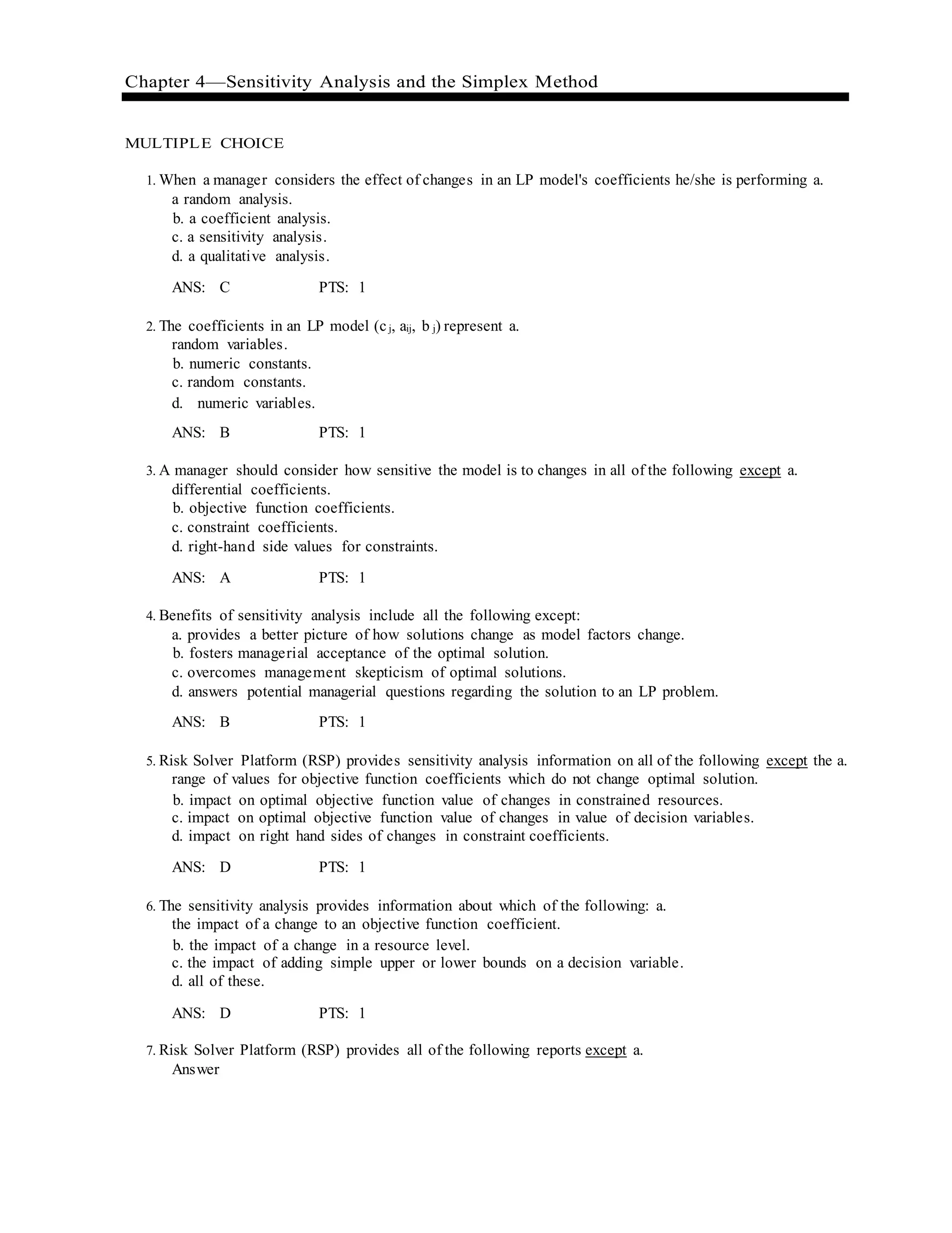
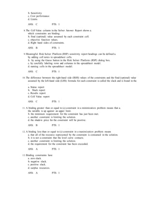
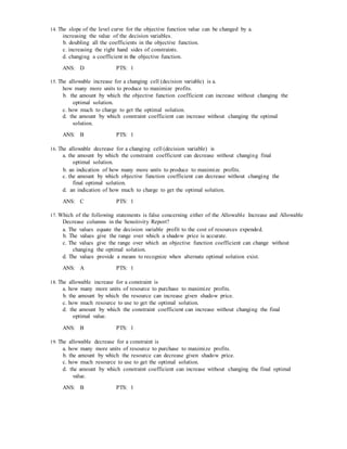
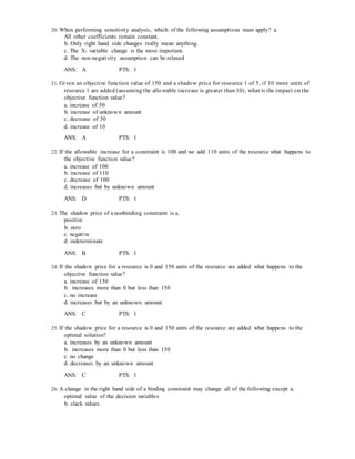
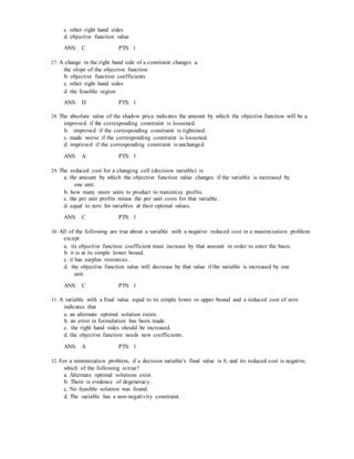
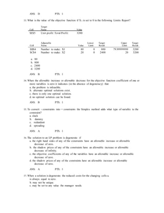
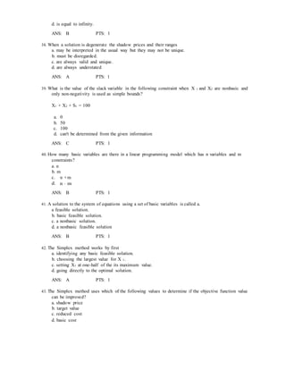
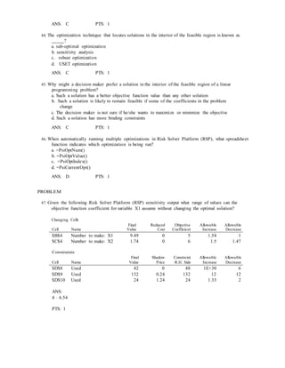
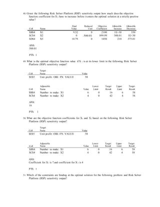
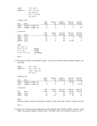
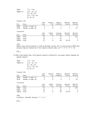
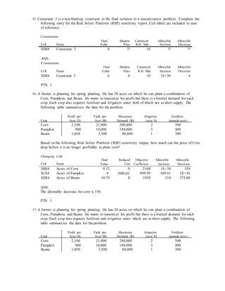
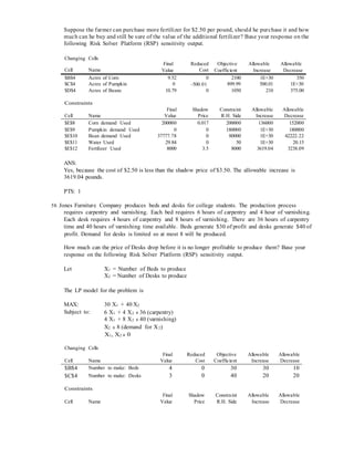
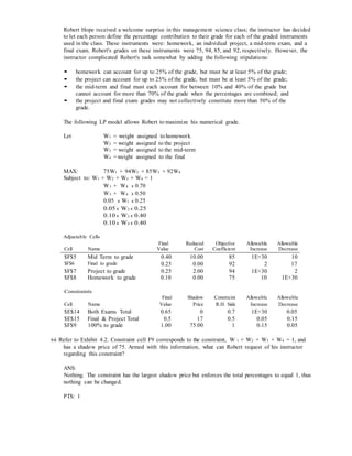
This document contains 50 multiple choice questions about sensitivity analysis and the simplex method for linear programming models. It covers topics like sensitivity analysis reports in Risk Solver Platform, shadow prices, reduced costs, allowable increases/decreases, and interpreting outputs to determine optimal objective function values or coefficients that will change the optimal solution. The questions provide examples of linear programming outputs and ask the test taker to interpret the results.

1. Chapter 4—Sensitivity Analysis and the Simplex Method
MULTIPLE CHOICE
1. When a manager considers the effect of changes in an LP model's coefficients he/she is performing a.
a random analysis.
b. a coefficient analysis.
c. a sensitivity analysis.
d. a qualitative analysis.
ANS: C PTS: 1
2. The coefficients in an LP model (cj, aij, b j) represent a.
random variables.
b. numeric constants.
c. random constants.
d. numeric variables.
ANS: B PTS: 1
3. A manager should consider how sensitive the model is to changes in all of the following except a.
differential coefficients.
b. objective function coefficients.
c. constraint coefficients.
d. right-hand side values for constraints.
ANS: A PTS: 1
4. Benefits of sensitivity analysis include all the following except:
a. provides a better picture of how solutions change as model factors change.
b. fosters managerial acceptance of the optimal solution.
c. overcomes management skepticism of optimal solutions.
d. answers potential managerial questions regarding the solution to an LP problem.
ANS: B PTS: 1
5. Risk Solver Platform (RSP) provides sensitivity analysis information on all of the following except the a.
range of values for objective function coefficients which do not change optimal solution.
b. impact on optimal objective function value of changes in constrained resources.
c. impact on optimal objective function value of changes in value of decision variables.
d. impact on right hand sides of changes in constraint coefficients.
ANS: D PTS: 1
6. The sensitivity analysis provides information about which of the following: a.
the impact of a change to an objective function coefficient.
b. the impact of a change in a resource level.
c. the impact of adding simple upper or lower bounds on a decision variable.
d. all of these.
ANS: D PTS: 1
7. Risk Solver Platform (RSP) provides all of the following reports except a.
Answer

2. b. Sensitivity
c. Cost performance
d. Limits
ANS: C PTS: 1
8. The Cell Value column in the Solver Answer Report shows a.
which constraints are binding.
b. final (optimal) value assumed by each constraint cell.
c. objective function values.
d. Right hand sides of constraints.
ANS: B PTS: 1
9. Meaningful Risk Solver Platform (RSP) sensitivity report headings can be defined a.
by adding cell notes to spreadsheet cells.
b. by using the Guess button in the Risk Solver Platform (RSP) dialog box.
c. by carefully labeling rows and columns in the spreadsheet model.
d. naming cells in the spreadsheet model.
ANS: C PTS: 1
10. The difference between the right-hand side (RHS) values of the constraints and the final (optimal) value
assumed by the left-hand side (LHS) formula for each constraint is called the slack and is found in the
.
a. Status report
b. Slack report
c. Results report
d. Cell Value report
ANS: C PTS: 1
11. A binding greater than or equal to (≥) constraint in a minimization problem means that a.
the variable is up against an upper limit.
b. the minimum requirement for the constraint has just been met.
c. another constraint is limiting the solution.
d. the shadow price for the constraint will be positive.
ANS: B PTS: 1
12. A binding less than or equal to (≤) constraint in a maximization problem means
a. that all of the resource represented by the constraint is consumed in the solution.
b. it is not a constraint that the level curve contacts.
c. another constraint is limiting the solution.
d. the requirement for the constraint has been exceeded.
ANS: A PTS: 1
13. Binding constraints have
a. zero slack.
b. negative slack.
c. positive slack.
d. surplus resources.
ANS: A PTS: 1

3. 14. The slope of the level curve for the objective function value can be changed by a.
increasing the value of the decision variables.
b. doubling all the coefficients in the objective function.
c. increasing the right hand sides of constraints.
d. changing a coefficient in the objective function.
ANS: D PTS: 1
15. The allowable increase for a changing cell (decision variable) is a.
how many more units to produce to maximize profits.
b. the amount by which the objective function coefficient can increase without changing the
optimal solution.
c. how much to charge to get the optimal solution.
d. the amount by which constraint coefficient can increase without changing the optimal
solution.
ANS: B PTS: 1
16. The allowable decrease for a changing cell (decision variable) is
a. the amount by which the constraint coefficient can decrease without changing final
optimal solution.
b. an indication of how many more units to produce to maximize profits.
c. the amount by which objective function coefficient can decrease without changing the
final optimal solution.
d. an indication of how much to charge to get the optimal solution.
ANS: C PTS: 1
17. Which of the following statements is false concerning either of the Allowable Increase and Allowable
Decrease columns in the Sensitivity Report?
a. The values equate the decision variable profit to the cost of resources expended.
b. The values give the range over which a shadow price is accurate.
c. The values give the range over which an objective function coefficient can change without
changing the optimal solution.
d. The values provide a means to recognize when alternate optimal solution exist.
ANS: A PTS: 1
18. The allowable increase for a constraint is
a. how many more units of resource to purchase to maximize profits.
b. the amount by which the resource can increase given shadow price.
c. how much resource to use to get the optimal solution.
d. the amount by which the constraint coefficient can increase without changing the final
optimal value.
ANS: B PTS: 1
19. The allowable decrease for a constraint is
a. how many more units of resource to purchase to maximize profits.
b. the amount by which the resource can decrease given shadow price.
c. how much resource to use to get the optimal solution.
d. the amount by which constraint coefficient can increase without changing the final optimal
value.
ANS: B PTS: 1

4. 20. When performing sensitivity analysis, which of the following assumptions must apply? a.
All other coefficients remain constant.
b. Only right hand side changes really mean anything.
c. The X1 variable change is the most important.
d. The non-negativity assumption can be relaxed
ANS: A PTS: 1
21. Given an objective function value of 150 and a shadow price for resource 1 of 5, if 10 more units of
resource 1 are added (assuming the allowable increase is greater than 10), what is the impact on the
objective function value?
a. increase of 50
b. increase of unknown amount
c. decrease of 50
d. increase of 10
ANS: A PTS: 1
22. If the allowable increase for a constraint is 100 and we add 110 units of the resource what happens to
the objective function value?
a. increase of 100
b. increase of 110
c. decrease of 100
d. increases but by unknown amount
ANS: D PTS: 1
23. The shadow price of a nonbinding constraint is a.
positive
b. zero
c. negative
d. indeterminate
ANS: B PTS: 1
24. If the shadow price for a resource is 0 and 150 units of the resource are added what happens to the
objective function value?
a. increase of 150
b. increases more than 0 but less than 150
c. no increase
d. increases but by an unknown amount
ANS: C PTS: 1
25. If the shadow price for a resource is 0 and 150 units of the resource are added what happens to the
optimal solution?
a. increases by an unknown amount
b. increases more than 0 but less than 150
c. no change
d. decreases by an unknown amount
ANS: C PTS: 1
26. A change in the right hand side of a binding constraint may change all of the following except a.
optimal value of the decision variables
b. slack values

5. c. other right hand sides
d. objective function value
ANS: C PTS: 1
27. A change in the right hand side of a constraint changes a.
the slope of the objective function
b. objective function coefficients
c. other right hand sides
d. the feasible region
ANS: D PTS: 1
28. The absolute value of the shadow price indicates the amount by which the objective function will be a.
improved if the corresponding constraint is loosened.
b. improved if the corresponding constraint is tightened.
c. made worse if the corresponding constraint is loosened.
d. improved if the corresponding constraint is unchanged.
ANS: A PTS: 1
29. The reduced cost for a changing cell (decision variable) is
a. the amount by which the objective function value changes if the variable is increased by
one unit.
b. how many more units to product to maximize profits.
c. the per unit profits minus the per unit costs for that variable.
d. equal to zero for variables at their optimal values.
ANS: C PTS: 1
30. All of the following are true about a variable with a negative reduced cost in a maximization problem
except
a. its objective function coefficient must increase by that amount in order to enter the basis.
b. it is at its simple lower bound.
c. it has surplus resources.
d. the objective function value will decrease by that value if the variable is increased by one
unit.
ANS: C PTS: 1
31. A variable with a final value equal to its simple lower or upper bound and a reduced cost of zero
indicates that
a. an alternate optimal solution exists.
b. an error in formulation has been made.
c. the right hand sides should be increased.
d. the objective function needs new coefficients.
ANS: A PTS: 1
32. For a minimization problem, if a decision variable's final value is 0, and its reduced cost is negative,
which of the following is true?
a. Alternate optimal solutions exist.
b. There is evidence of degeneracy.
c. No feasible solution was found.
d. The variable has a non-negativity constraint.

6. ANS: D PTS: 1
33. What is the value of the objective function if X 1 is set to 0 in the following Limits Report?
Target
Cell Name Value
$E$5 Unit profit: Total Profit: 3200
Cell
Adjustable
Name Value
Lower
Limit
Target
Result
Upper
Limit
Target
Result
$B$4 Number to make: X1 80 0 800 79.99999999 3200
$C$4 Number to make: X2 20 0 2400 20 3200
a. 80
b. 800
c. 2400
d. 3200
ANS: B PTS: 1
34. When the allowable increase or allowable decrease for the objective function coefficient of one or
more variables is zero it indicates (in the absence of degeneracy) that
a. the problem is infeasible.
b. alternate optimal solutions exist.
c. there is only one optimal solution.
d. no optimal solution can be found.
ANS: B PTS: 1
35. To convert ≤ constraints into = constraints the Simplex method adds what type of variable to the
constraint?
a. slack
b. dummy
c. redundant
d. spreading
ANS: A PTS: 1
36. The solution to an LP problem is degenerate if
a. the right hand sides of any of the constraints have an allowable increase or allowable
decrease of zero.
b. the shadow prices of any of the constraints have an allowable increase or allowable
decrease of infinity.
c. the objective coefficients of any of the variables have an allowable increase or allowable
decrease of zero.
d. the shadow prices of any of the constraints have an allowable increase or allowable
decrease of zero.
ANS: A PTS: 1
37. When a solution is degenerate the reduced costs for the changing cells a.
is always equal to zero.
b. may not be unique.
c. may be set to any value the manager needs.

7. d. is equal to infinity.
ANS: B PTS: 1
38. When a solution is degenerate the shadow prices and their ranges
a. may be interpreted in the usual way but they may not be unique.
b. must be disregarded.
c. are always valid and unique.
d. are always understated
ANS: A PTS: 1
39. What is the value of the slack variable in the following constraint when X 1 and X2 are nonbasic and
only non-negativity is used as simple bounds?
X1 + X2 + S1 = 100
a. 0
b. 50
c. 100
d. can't be determined from the given information
ANS: C PTS: 1
40. How many basic variables are there in a linear programming model which has n variables and m
constraints?
a. n
b. m
c. n + m
d. n − m
ANS: B PTS: 1
41. A solution to the system of equations using a set of basic variables is called a.
a feasible solution.
b. basic feasible solution.
c. a nonbasic solution.
d. a nonbasic feasible solution
ANS: B PTS: 1
42. The Simplex method works by first
a. identifying any basic feasible solution.
b. choosing the largest value for X 1.
c. setting X1 at one-half of the its maximum value.
d. going directly to the optimal solution.
ANS: A PTS: 1
43. The Simplex method uses which of the following values to determine if the objective function value
can be improved?
a. shadow price
b. target value
c. reduced cost
d. basic cost

8. ANS: C PTS: 1
44. The optimization technique that locates solutions in the interior of the feasible region is known as
?
a. sub-optimal optimization
b. sensitivity analysis
c. robust optimization
d. USET optimization
ANS: C PTS: 1
45. Why might a decision maker prefer a solution in the interior of the feasible region of a linear
programming problem?
a. Such a solution has a better objective function value than any other solution
b. Such a solution is likely to remain feasible if some of the coefficients in the problem
change
c. The decision maker is not sure if he/she wants to maximize or minimize the objective
d. Such a solution has more binding constraints
ANS: C PTS: 1
46. When automatically running multiple optimizations in Risk Solver Platform (RSP), what spreadsheet
function indicates which optimization is being run?
a. =PsiOptNum()
b. =PsiOptValue()
c. =PsiOptIndex()
d. =PsiCurrentOpt()
ANS: D PTS: 1
PROBLEM
47. Given the following Risk Solver Platform (RSP) sensitivity output what range of values can the
objective function coefficient for variable X1 assume without changing the optimal solution?
Changing Cells
Cell Name
Final
Value
Reduced
Cost
Objective
Coefficient
Allowable
Increase
Allowable
Decrease
$B$4 Number to make: X1 9.49 0 5 1.54 1
$C$4 Number to make: X2 1.74 0 6 1.5 1.47
Constraints
Final Shadow Constraint Allowable Allowable
Cell Name Value Price R.H. Side Increase Decrease
$D$8 Used 42 0 48 1E+30 6
$D$9 Used 132 0.24 132 12 12
$D$10 Used 24 1.24 24 1.33 2
ANS:
4 − 6.54
PTS: 1

9. 48. Given the following Risk Solver Platform (RSP) sensitivity output how much does the objective
function coefficient for X 2 have to increase before it enters the optimal solution at a strictly positive
value?
Cell Name
Final
Value
Reduced
Cost
Objective
Coefficient
Allowable
Increase
Allowable
Decrease
$B$4 X1 9.52 0 2100 1E+30 350
$C$4 X2 0 −500.01 899.99 500.01 1E+30
$D$4 X3 10.79 0 1050 210 375.01
ANS:
500.01
PTS: 1
49. What is the optimal objective function value if X 1 is at its lower limit in the following Risk Solver
Platform (RSP) sensitivity output?
Target
Cell Name Value
$E$5 Unit profit: OBJ. FN. VALUE 58
Cell
Adjustable
Name Value
Lower
Limit
Target
Result
Upper
Limit
Target
Result
$B$4 Number to make: X1 6 0 16 6 58
$C$4 Number to make: X2 4 0 42 4 58
ANS:
16
PTS: 1
50. What are the objective function coefficients for X1 and X2 based on the following Risk Solver
Platform (RSP) sensitivity output?
Target
Cell Name Value
$E$5 Unit profit: OBJ. FN. VALUE 58
Cell
Adjustable
Name Value
Lower
Limit
Target
Result
Upper
Limit
Target
Result
$B$4 Number to make: X1 6 0 16 6 58
$C$4 Number to make: X2 4 0 42 4 58
ANS:
Coefficient for X1 is 7 and coefficient for X 2 is 4
PTS: 1
51. Which of the constraints are binding at the optimal solution for the following problem and Risk Solver
Platform (RSP) sensitivity output?

10. MAX: 7 X1 + 4 X2
Subject to: 2 X1 + X2 ≤ 16
X1 + X2 ≤ 10
2 X1 + 5 X2 ≤ 40
X1, X2 ≥ 0
Changing Cells
Final Reduced Objective Allowable Allowable
Cell Name Value Cost Coefficient Increase Decrease
$B$4 Number to make: X1 6 0 7 1 3
$C$4 Number to make: X2 4 0 4 3 0.5
Constraints
Final Shadow Constraint Allowable Allowable
Cell Name Value Price R.H. Side Increase Decrease
$D$8 Used 16 3 16 4 2.67
$D$9 Used 10 1 10 1 2
$D$10 Used 32 0 40 1E+30 8
ANS:
X1 = 6, X2 = 4
2 * 6 + 4 = 16 binding
6 + 4 = 10 binding
2 * 6 + 5 * 4 = 32 non-binding
PTS: 1
52. Is the optimal solution to this problem unique, or is there an alternate optimal solution? Explain your
reasoning.
MAX 5 X1 + 2 X2
Subject to: 3 X1 + 5 X2 ≤ 15
10 X1 + 4 X2 ≤ 20
X1, X2 ≥ 0
Changing Cells
Final Reduced Objective Allowable Allowable
Cell Name Value Cost Coefficient Increase Decrease
$B$4 Number to make: X1 2 0 5 1E+30 0
$C$4 Number to make: X2 0 0 2 0 1E+30
Constraints
Final Shadow Constraint Allowable Allowable
Cell Name Value Price R.H. Side Increase Decrease
$D$8 Used 6 0 15 1E+30 9
$D$9 Used 20 0.5 20 30 20
ANS:
Alternate optimal solutions exist because variable X 2 has a final value of 0 and a reduced cost of 0.
PTS: 1
53. Consider the following linear programming model and Risk Solver Platform (RSP) sensitivity output.
What is the optimal objective function value if the RHS of the first constraint increases to 18?

11. MAX: 7 X1 + 4 X2
Subject to: 2 X1 + X2 ≤ 16
X1 + X2 ≤ 10
2 X1 + 5 X2 ≤ 40
X1, X2 ≥ 0
Changing Cells
Final Reduced Objective Allowable Allowable
Cell Name Value Cost Coefficient Increase Decrease
$B$4 Number to make: X1 6 0 7 1 3
$C$4 Number to make: X2 4 0 4 3 0.5
Constraints
Final Shadow Constraint Allowable Allowable
Cell Name Value Price R.H. Side Increase Decrease
$D$8 Used 16 3 16 4 2.67
$D$9 Used 10 1 10 1 2
$D$10 Used 32 0 40 1E+30 8
ANS:
Shadow price of first constraint is 3 with an allowable increase of 4. A 2-unit increase in RHS value
increases objective function by 6. New objective function value is 6 * 7 + 4 * 4 + 2 * 3 = 64.
PTS: 1
54. What is the smallest value of the objective function coefficient X 1 can assume without changing the
optimal solution?
MAX: 7 X1 + 4 X2
Subject to: 2 X1 + X2 ≤ 16
X1 + X2 ≤ 10
2 X1 + 5 X2 ≤ 40
X1, X2 ≥ 0
Changing Cells
Final Reduced Objective Allowable Allowable
Cell Name Value Cost Coefficient Increase Decrease
$B$4 Number to make: X1 6 0 7 1 3
$C$4 Number to make: X2 4 0 4 3 0.5
Constraints
Final Shadow Constraint Allowable Allowable
Cell Name Value Price R.H. Side Increase Decrease
$D$8 Used 16 3 16 4 2.67
$D$9 Used 10 1 10 1 2
$D$10 Used 32 0 40 1E+30 8
ANS:
Coefficient − allowable decrease = 7 − 3 = 4
PTS: 1

12. Profit per Yield per Maximum Irrigation Fertilizer
Profit per Yield per Maximum Irrigation Fertilizer
55. Constraint 3 is a non-binding constraint in the final solution to a maximization problem. Complete the
following entry for the Risk Solver Platform (RSP) sensitivity report. Cell labels are included to ease
of reference.
Constraints
Cell Name
Final
Value
Shadow
Price
Constraint
R.H. Side
Allowable
Increase
Allowable
Decrease
$D$8 Constraint 3 6 ?? 10 ?? ??
ANS:
Constraints
Final Shadow Constraint Allowable Allowable
Cell Name Value Price R.H. Side Increase Decrease
$D$8 Constraint 3 6 0 10 1E+30 4
PTS: 1
56. A farmer is planning his spring planting. He has 20 acres on which he can plant a combination of
Corn, Pumpkins and Beans. He wants to maximize his profit but there is a limited demand for each
crop. Each crop also requires fertilizer and irrigation water both of which are in short supply. The
following table summarizes the data for the problem.
Crop Acre ($) Acre (lb) Demand (lb) (acre ft) (pounds/acre)
Corn 2,100 21,000 200,000 2 500
Pumpkin 900 10,000 180,000 3 400
Beans 1,050 3,500 80,000 1 300
Based on the following Risk Solver Platform (RSP) sensitivity output, how much can the price of Corn
drop before it is no longer profitable to plant corn?
Changing Cells
Cell Name
Final
Value
Reduced
Cost
Objective
Coefficient
Allowable
Increase
Allowable
Decrease
$B$4 Acres of Corn 9.52 0 2100 1E+30 350
$C$4 Acres of Pumpkin 0 −500.01 899.99 500.01 1E+30
$D$4 Acres of Beans 10.79 0 1050 210 375.00
ANS:
The allowable decrease for corn is 350.
PTS: 1
57. A farmer is planning his spring planting. He has 20 acres on which he can plant a combination of
Corn, Pumpkins and Beans. He wants to maximize his profit but there is a limited demand for each
crop. Each crop also requires fertilizer and irrigation water which are in short supply. The following
table summarizes the data for the problem.
Crop Acre ($) Acre (lb) Demand (lb) (acre ft) (pounds/acre)
Corn 2,100 21,000 200,000 2 500
Pumpkin 900 10,000 180,000 3 400
Beans 1,050 3,500 80,000 1 300

13. Suppose the farmer can purchase more fertilizer for $2.50 per pound, should he purchase it and how
much can he buy and still be sure of the value of the additional fertilizer? Base your response on the
following Risk Solver Platform (RSP) sensitivity output.
Changing Cells
Cell Name
Final
Value
Reduced
Cost
Objective
Coefficient
Allowable
Increase
Allowable
Decrease
$B$4 Acres of Corn 9.52 0 2100 1E+30 350
$C$4 Acres of Pumpkin 0 −500.01 899.99 500.01 1E+30
$D$4 Acres of Beans 10.79 0 1050 210 375.00
Constraints
Final Shadow Constraint Allowable Allowable
Cell Name Value Price R.H. Side Increase Decrease
$E$8 Corn demand Used 200000 0.017 200000 136000 152000
$E$9 Pumpkin demand Used 0 0 180000 1E+30 180000
$E$10 Bean demand Used 37777.78 0 80000 1E+30 42222.22
$E$11 Water Used 29.84 0 50 1E+30 20.15
$E$12 Fertilizer Used 8000 3.5 8000 3619.04 3238.09
ANS:
Yes, because the cost of $2.50 is less than the shadow price of $3.50. The allowable increase is
3619.04 pounds.
PTS: 1
58. Jones Furniture Company produces beds and desks for college students. The production process
requires carpentry and varnishing. Each bed requires 6 hours of carpentry and 4 hour of varnishing.
Each desk requires 4 hours of carpentry and 8 hours of varnishing. There are 36 hours of carpentry
time and 40 hours of varnishing time available. Beds generate $30 of profit and desks generate $40 of
profit. Demand for desks is limited so at most 8 will be produced.
How much can the price of Desks drop before it is no longer profitable to produce them? Base your
response on the following Risk Solver Platform (RSP) sensitivity output.
Let X1 = Number of Beds to produce
X2 = Number of Desks to produce
The LP model for the problem is
MAX: 30 X1 + 40 X2
Subject to: 6 X1 + 4 X2 ≤ 36 (carpentry)
4 X1 + 8 X2 ≤ 40 (varnishing)
X2 ≤ 8 (demand for X2)
X1, X2 ≥ 0
Changing Cells
Final Reduced Objective Allowable Allowable
Cell Name Value Cost Coefficient Increase Decrease
$B$4 Number to make: Beds 4 0 30 30 10
$C$4 Number to make: Desks 3 0 40 20 20
Constraints
Final Shadow Constraint Allowable Allowable
Cell Name Value Price R.H. Side Increase Decrease

14. $D$8 Carpentry Used 36 2.5 36 24 16
$D$9 Varnishing Used 40 3.75 40 26.67 16
$D$10 Desk demand Used 3 0 8 1E+30 5
ANS:
The allowable decrease is 20.
PTS: 1
59. Jones Furniture Company produces beds and desks for college students. The production process
requires carpentry and varnishing. Each bed requires 6 hours of carpentry and 4 hour of varnishing.
Each desk requires 4 hours of carpentry and 8 hours of varnishing. There are 36 hours of carpentry
time and 40 hours of varnishing time available. Beds generate $30 of profit and desks generate $40 of
profit. Demand for desks is limited so at most 8 will be produced.
Suppose the company can purchase more varnishing time for $3.00, should it be purchased and how
much can be bought before the value of the additional time is uncertain? Base your response on the
following Risk Solver Platform (RSP) sensitivity output.
Let X1 = Number of Beds to produce
X2 = Number of Desks to produce
The LP model for the problem is
MAX: 30 X1 + 40 X2
Subject to: 6 X1 + 4 X2 ≤ 36 (carpentry)
4 X1 + 8 X2 ≤ 40 (varnishing)
X2 ≤ 8 (demand for X2)
X1, X2 ≥ 0
Changing Cells
Cell Name
Final
Value
Reduced
Cost
Objective
Coefficient
Allowable
Increase
Allowable
Decrease
$B$4 Number to make: Beds 4 0 30 30 10
$C$4 Number to make: Desks 3 0 40 20 20
Constraints
Final Shadow Constraint Allowable Allowable
Cell Name Value Price R.H. Side Increase Decrease
$D$8 Carpentry Used 36 2.5 36 24 16
$D$9 Varnishing Used 40 3.75 40 26.67 16
$D$10 Desk demand Used 3 0 8 1E+30 5
ANS:
Yes, because the cost of $3.00 is less than the shadow price of $3.75. The allowable increase is 26.67
hours.
PTS: 1
Exhibit 4.1
The following questions are based on the problem below and accompanying Risk Solver Platform
(RSP) sensitivity report.

15. Carlton construction is supplying building materials for a new mall construction project in Kansas.
Their contract calls for a total of 250,000 tons of material to be delivered over a three-week period.
Carlton's supply depot has access to three modes of transportation: a trucking fleet, railway delivery,
and air cargo transport. Their contract calls for 120,000 tons delivered by the end of week one, 80% of
the total delivered by the end of week two, and the entire amount delivered by the end of week three.
Contracts in place with the transportation companies call for at least 45% of the total delivered be
delivered by trucking, at least 40% of the total delivered be delivered by railway, and up to 15% of the
total delivered be delivered by air cargo. Unfortunately, competing demands limit the availability of
each mode of transportation each of the three weeks to the following levels (all in thousands of tons):
Week Trucking Limits Railway Limits Air Cargo Limits
1 45 60 15
2 50 55 10
3 55 45 5
Costs ($ per 1000 tons) $200 $140 $400
The following is the LP model for this logistics problem.
Let Xij = amount shipped by mode i in week j
where i = 1(Truck), 2(Rail), 3(Air)
and j = 1, 2, 3
Let WLij = weekly limit of mode i in week j (as provided in above table)
MIN: 200(X11 + X12 + X13) + 140(X21 + X22 + X23) + 500(X31 + X32 + X33)
Subject to:
Xij ≤ WL ij for all i and j Weekly limits by mode
X11 + X12 + X13 + X21 + X22 + X23 + X31 + X32 + X33 ≥ 250 Total at end of three weeks
X11 + X21 + X31 + X12 + X22 + X32 ≥ 200 Total at end of two weeks
X11 + X21 + X31 ≥ 120 Total at end of first week
X11 + X12 +X13 ≥ 0.45*250 Truck mix requirement
X21 + X22 +X23 ≥ 0.40*250 Rail mix requirement
X31 + X32 + X33 ≤ 0.15*250 Air mix limit
Xij ≥ 0 for all i and j
Cell Name
Final
Value
Reduced
Cost
Objective
Coefficient
Allowable
Increase
Allowable
Decrease
$D$6 Week 1 by Truck 45 0 200 360 1E+30
$E$6 Week 1 by Rail 60 0 140 360 1E+30
$F$6 Week 1 by Air 15 0 500 1E+30 360
$D$7 Week 2 by Truck 50 0 200 0 1E+30
$E$7 Week 2 by Rail 55 0 140 0 1E+30
$F$7 Week 2 by Air 0 360 500 1E+30 360
$D$8 Week 3 by Truck 13 0 200 1E+30 0
$E$8 Week 3 by Rail 12 0 140 60 0
$F$8 Week 3 by Air 0 360 500 1E+30 360
Constraints
Final Shadow Constraint Allowable Allowable
Cell Name Value Price R.H. Side Increase Decrease
$D$18 Week 1 by Truck 45 −360 45 13 0
$E$18 Week 1 by Rail 60 −360 60 15 0
$F$18 Week 1 by Air 15 0 15 1E+30 0

16. $D$19 Week 2 by Truck 50 0 50 13 25
$E$19 Week 2 by Rail 55 0 55 12 25
$F$19 Week 2 by Air 0 0 10 1E+30 10
$D$20 Week 3 by Truck 13 0 55 1E+30 42
$E$20 Week 3 by Rail 12 0 45 1E+30 33
$F$20 Week 3 by Air 0 0 5 1E+30 5
$D$9 Shipped by Truck 108 60 108 12 13
$E$9 Shipped by Rail 127 0 100 27 1E+30
$F$13 Total Shipped Tons 250 140 250 33 0
$F$9 Shipped by Air 15 0 37.5 1E+30 22.5
$G$6 Week 1 Totals 120 360 120 0 15
$G$7 Week 2 Totals 225 0 200 25 1E+30
$G$8 Week 3 Totals 250 0 250 0 1E+30
60. Refer to Exhibit 4.1. The Week 1 by Truck and Week 1 by Rail constraints each have a shadow price of
−360. What do these values imply?
ANS:
Increase the weekly limits on these two modes to reduce total cost by $360 per unit increase in limit.
PTS: 1
61. Refer to Exhibit 4.1. Of the three percentage of effort constraints, Shipped by Truck, Shipped by Rail,
and Shipped by Air, which should be examined for potential cost reduction?
ANS:
The percentage by Truck, Shipped by Truck, should be examined. Decreasing the percentage by truck
(from 45%) will decrease cost as the shadow price is 60.
PTS: 1
62. Refer to Exhibit 4.1. Are there alternate optimal solutions to this problem?
ANS:
Cannot tell because we cannot rule out degeneracy according to our guidelines due to the zero values
in the Allowable Increase and Allowable Decrease columns of the constraint portion of the Risk Solver
Platform (RSP) sensitivity report.
PTS: 1
63. Refer to Exhibit 4.1. Should the company negotiate for additional air delivery capacity?
ANS:
No. The shadow prices for each week of air delivery are zero.
PTS: 1
Exhibit 4.2
The following questions correspond to the problem below and associated Risk Solver Platform (RSP)
sensitivity report.

17. Robert Hope received a welcome surprise in this management science class; the instructor has decided
to let each person define the percentage contribution to their grade for each of the graded instruments
used in the class. These instruments were: homework, an individual project, a mid-term exam, and a
final exam. Robert's grades on these instruments were 75, 94, 85, and 92, respectively. However, the
instructor complicated Robert's task somewhat by adding the following stipulations:
• homework can account for up to 25% of the grade, but must be at least 5% of the grade;
• the project can account for up to 25% of the grade, but must be at least 5% of the grade;
• the mid-term and final must each account for between 10% and 40% of the grade but
cannot account for more than 70% of the grade when the percentages are combined; and
• the project and final exam grades may not collectively constitute more than 50% of the
grade.
The following LP model allows Robert to maximize his numerical grade.
Let W1 = weight assigned to homework
W2 = weight assigned to the project
W3 = weight assigned to the mid-term
W4 =weight assigned to the final
MAX: 75W1 + 94W2 + 85W3 + 92W4
Subject to: W1 + W2 + W3 + W4 = 1
W3 + W4 ≤ 0.70
W3 + W4 ≥ 0.50
0.05 ≤ W1 ≤ 0.25
0.05 ≤ W2 ≤ 0.25
0.10 ≤ W3 ≤ 0.40
0.10 ≤ W4 ≤ 0.40
Adjustable Cells
Cell Name
Final
Value
Reduced
Cost
Objective
Coefficient
Allowable
Increase
Allowable
Decrease
$F$5 Mid Term to grade 0.40 10.00 85 1E+30 10
$F$6 Final to grade 0.25 0.00 92 2 17
$F$7 Project to grade 0.25 2.00 94 1E+30 2
$F$8 Homework to grade 0.10 0.00 75 10 1E+30
Constraints
Final Shadow Constraint Allowable Allowable
Cell Name Value Price R.H. Side Increase Decrease
$E$14 Both Exams Total 0.65 0 0.7 1E+30 0.05
$E$15 Final & Project Total 0.5 17 0.5 0.05 0.15
$F$9 100% to grade 1.00 75.00 1 0.15 0.05
64. Refer to Exhibit 4.2. Constraint cell F9 corresponds to the constraint, W 1 + W2 + W3 + W4 = 1, and
has a shadow price of 75. Armed with this information, what can Robert request of his instructor
regarding this constraint?
ANS:
Nothing. The constraint has the largest shadow price but enforces the total percentages to equal 1, thus
nothing can be changed.
PTS: 1

18. 65. Refer to Exhibit 4.2. Based on the Risk Solver Platform (RSP) sensitivity report information, is there
anything Robert can request of his instructor to improve his final grade?
ANS:
Robert can request an increase in the total weight allowed for the project and final exam combined
since this has a positive shadow price.
PTS: 1
66. Refer to Exhibit 4.2. Based on the Risk Solver Platform (RSP) sensitivity report information, Robert
has been approved by his instructor to increase the total weight allowed for the project and final exam
to 0.50 plus the allowable increase. When Robert re-solves his model, what will his new final grade
score be?
ANS:
88.85 since shadow price of 17 and increase of 0.05 equates to 0.85.
PTS: 1
67. Use slack variables to rewrite this problem so that all its constraints are equality constraints.
MAX: 2 X1 + 7 X2
Subject to: 5 X1 + 9 X2 ≤ 90
9 X1 + 8 X2 ≤ 144
X2 ≤ 8
X1, X2 ≥ 0
ANS:
MAX: 2 X1 + 7 X2
Subject to: 5 X1 + 9 X2 + S1 = 90
9 X1 + 8 X2 + S2 =144
X2 + S3 = 8
X1, X2 ≥ 0
PTS: 1
68. Identify the different sets of basic variables that might be used to obtain a solution to this problem.
MAX: 8 X1 + 4 X2
Subject to: 5 X1 + 5 X2 ≤ 20
6 X1 + 2 X2 ≤ 18
X1, X2 ≥ 0
ANS:
X1 X2 S1 S2
0 0 20 18
0 4 0 10
3 0 5 0
2.5 1.5 0 0
PTS: 1

19. 69. Use slack variables to rewrite this problem so that all its constraints are equality constraints.
MIN: 2.5 X1 + 1.5 X2
Subject to: 4 X1 + 3 X2 ≥ 24
2 X1 + 4 X2 ≥ 24
X1, X2 ≥ 0
ANS:
MIN 2.5 X1 + 1.5 X2
Subject to: 4 X1 + 3 X2 − S1 = 24
2 X1 + 4 X2 − S2 = 24
X1, X2 ≥ 0
PTS: 1
70. Identify the different sets of basic variables that might be used to obtain a solution to this problem.
MIN: 2.5 X1 + 1.5 X2
Subject to: 4 X1 + 3 X2 ≥ 24
2 X1 + 4 X2 ≥ 24
X1, X2 ≥ 0
ANS:
X1 X2 S1 S2
0 0 24 24
0 8 0 8
12 0 24 0
2.4 4.8 0 0
PTS: 1
71. Solve this problem graphically. What is the optimal solution and what constraints are binding at the
optimal solution?
MAX: 8 X1 + 4 X2
Subject to: 5 X1 + 5 X2 ≤ 20
6 X1 + 2 X2 ≤ 18
X1, X2 ≥ 0
ANS:
Obj = 26
X1 = 2.5
X2 = 1.5
Both constraints are binding.
PTS: 1
72. Solve this problem graphically. What is the optimal solution and what constraints are binding at the
optimal solution?

20. MIN: 7 X1 + 3 X2
Subject to: 4 X1 + 4 X2 ≥ 40
2 X1 + 3 X2 ≥ 24
X1, X2 ≥ 0
ANS:
Obj = 30
X1 = 0
X2 = 10
The constraint 4 X1 + 4 X2 = 40 is binding
PTS: 1