Downloaded 2,032 times
![M o s t a f a A l M a h m u d | 5
1. Continuity equation
𝝏𝒖
𝝏𝒙
+
𝝏𝒗
𝝏𝒚
= 𝟎 [
𝝏𝒘
𝝏𝒛
= 𝟎 → 𝟐𝒅 ]
2. x- direction Navier-Stokes equation
𝝆 (𝒖
𝝏𝒖
𝝏𝒙
+ 𝒗
𝝏𝒖
𝝏𝒚
) = −
𝝏𝒑
𝝏𝒙
+ 𝝁 (
𝝏 𝟐
𝒖
𝝏𝒙 𝟐
+
𝝏 𝟐
𝒖
𝝏𝒚 𝟐
)
3. y-direction Navier-Stokes equation:
𝝆 (𝒖
𝝏𝒗
𝝏𝒙
+ 𝒗
𝝏𝒗
𝝏𝒚
) = −
𝝏𝒑
𝝏𝒚
+ 𝝁 (
𝝏 𝟐
𝒗
𝝏𝒙 𝟐
+
𝝏 𝟐
𝒗
𝝏𝒚 𝟐
)
𝝏𝒖
𝝏𝒕
= 𝟎 → 𝐒𝐭𝐞𝐚𝐝𝐲
𝒘
𝝏𝒖
𝝏𝒛
= 𝟎; 𝒘
𝝏𝒗
𝝏𝒛
= 𝟎;
𝝏 𝟐
𝒖
𝝏𝒛 𝟐
= 𝟎 ;
𝝏 𝟐
𝒗
𝝏𝒛 𝟐
= 𝟎 → 𝟐𝑫
𝝆𝒈 𝒙 = 𝟎 ; 𝝆𝒈 𝒚 = 𝟎 → 𝐈𝐧𝐜𝐨𝐦𝐩𝐫𝐞𝐬𝐬𝐢𝐛𝐥𝐞
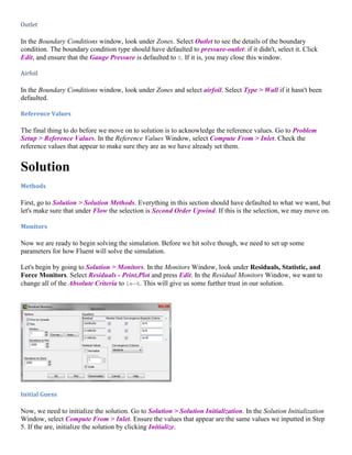
BOUNDARY CONDITIONS
Inlet velocity 0.25 m/s
For 2o
x-component 0.25 × cos(2 𝑜) = 0.2498477068
y-component 0.25 × sin(2 𝑜) = 0.008724874176
For 14o
x-component 0.25 × cos(14 𝑜) = 0.2425739316
y-component 0.25 × cos(14 𝑜) = 0.0604804739
Gage pressure at the inlet and outlet 0
Airfoil type Wall
Domain C- Mesh.](https://image.slidesharecdn.com/8ed4fe82-3382-40b5-9c0c-2936148b81b7-150128121551-conversion-gate01/85/CFD-analysis-of-an-Airfoil-6-320.jpg)
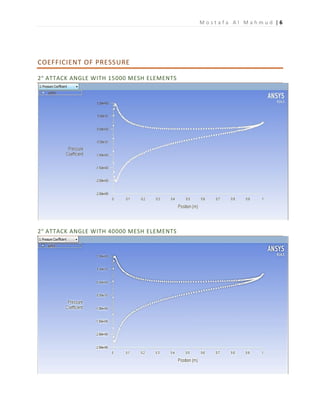
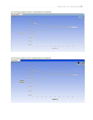
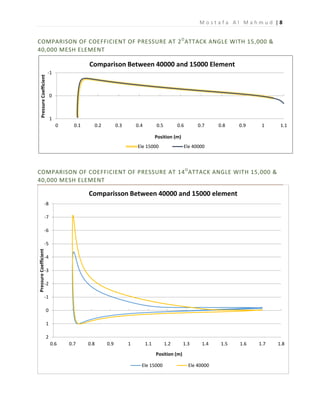
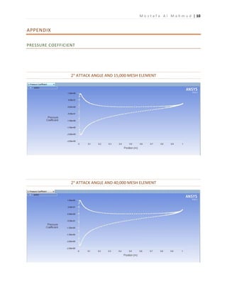
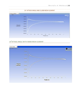
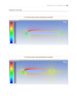
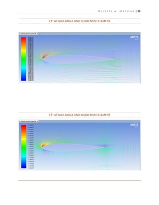
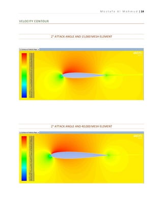
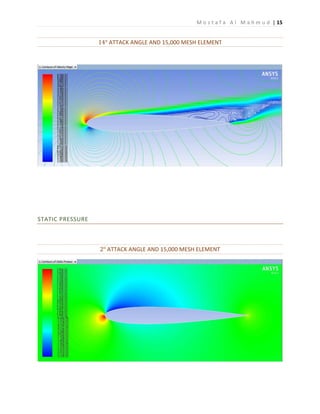
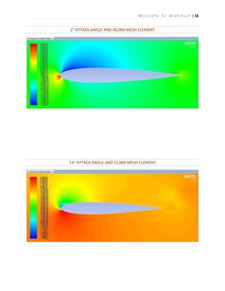
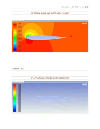
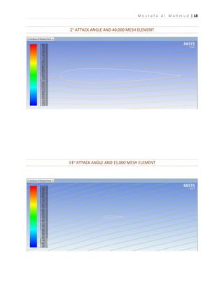
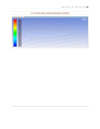
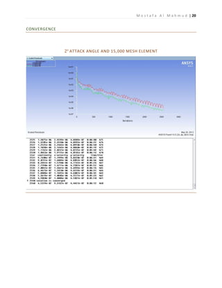
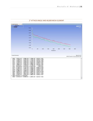
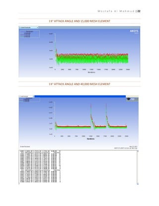
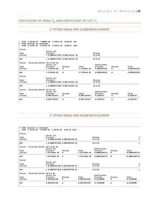
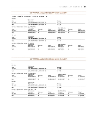
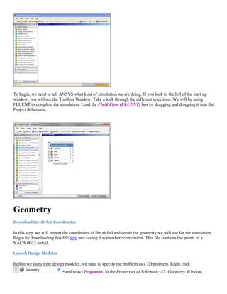
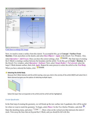
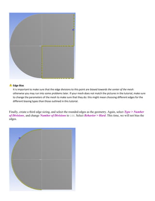
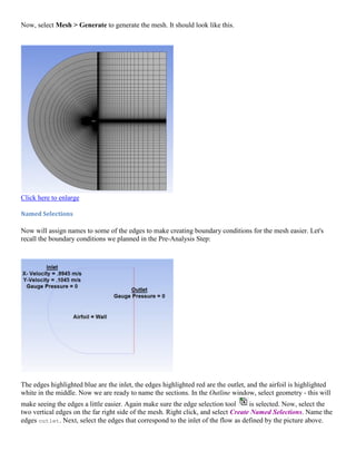
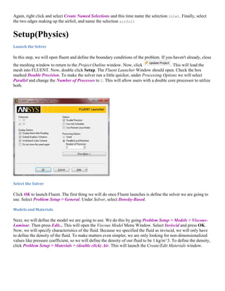
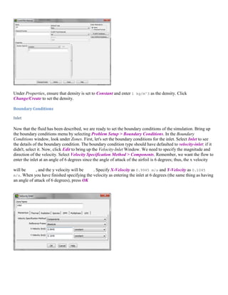

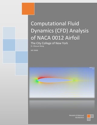
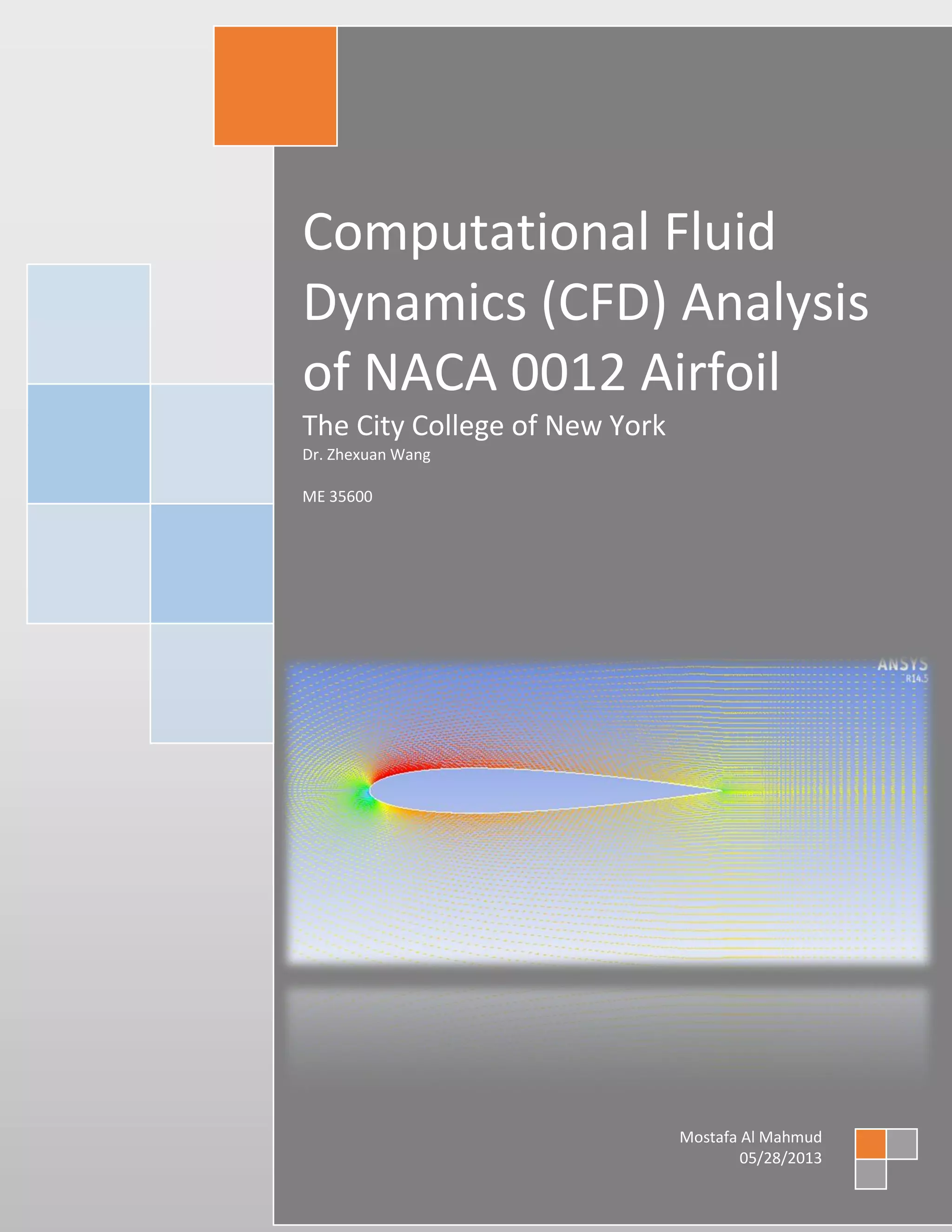
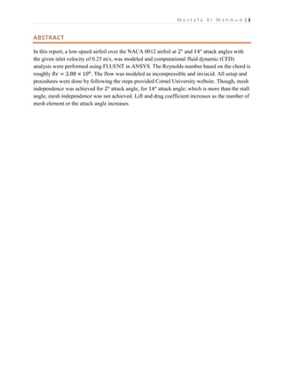
This document summarizes a computational fluid dynamics (CFD) analysis of flow over a NACA 0012 airfoil at attack angles of 2 and 14 degrees. Meshes with 15,000 and 40,000 elements were tested, with lift and drag coefficients increasing with higher mesh resolution and attack angle. Pressure contours, velocity vectors, and other flow visualizations were obtained from the CFD simulations in ANSYS. While mesh independence was achieved at 2 degrees, it was not at 14 degrees, which is above the airfoil's stall angle.