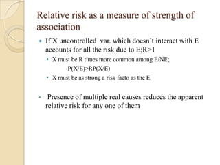
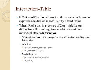
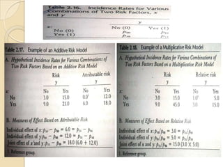
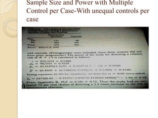
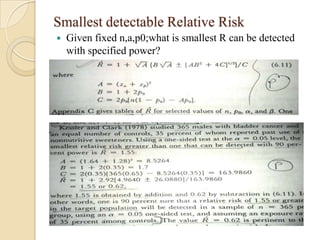
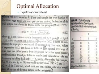
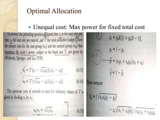
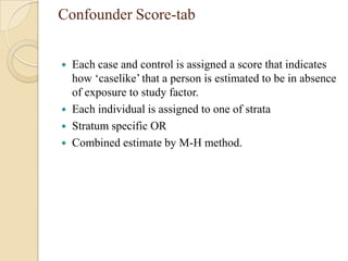
Downloaded 237 times


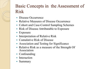
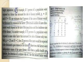
![Etiologic Fraction –Table1
λ =proportion of all cases in the target population
attributable to exposure.
λ =N1-Np2/N1
λ= pe(R-1)/[pe(R-1)+1]
eg-Table
p2=p(1- λ); p1= Rp(1- λ)
](https://image.slidesharecdn.com/casecontrolstudy-partii-140109231448-phpapp02/85/Case-control-study-Part-2-14-320.jpg)
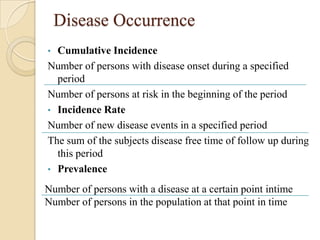
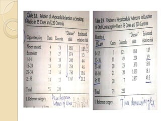
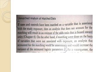
![Exposure-table
Intensity dimension
Time dimension
Estimation of Population Exposure Rate From Control
Series
Control series must be representative of individual without dis. In
target population
Dis. must be rare.
Unconditional prob of ex in target population=weighted
avg of cond.prob of ex among dis. and non-dis.
P(E)= P(E/D)P(D)+P(E/D̅)P(D̅)
If P(D) ≈0,P(D̅) ≈1; P(E)=P(E/D̅) ,(rare- pê ,̂̂ Ψ )
λ̂= pê (̂̂Ψ -1)/[pê (̂̂ Ψ -1)+1]
](https://image.slidesharecdn.com/casecontrolstudy-partii-140109231448-phpapp02/85/Case-control-study-Part-2-16-320.jpg)


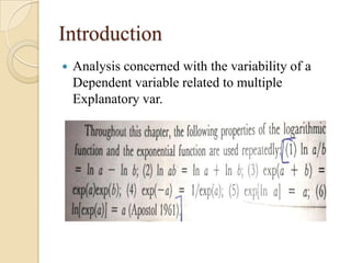
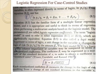


This document provides an outline and overview of key concepts in case-control study design and analysis. It discusses topics such as measures of disease occurrence, relative risk, sample size calculation, methods for adjusting for confounding, and multivariate analysis techniques including logistic regression and log-linear models. The goal is to introduce the basic methodology for case-control studies and analyzing associations between disease outcomes and exposures of interest.


![PERI-PROSTHETIC FRACTURE NAIL-PLATE CONSTRUCT [NPC].pptx](https://cdn.slidesharecdn.com/ss_thumbnails/drarunkumardrmohamedashrafperiprostheticfrasturenail-plateconstructnpc-260209164459-7e9d15a1-thumbnail.jpg?width=640&height=640&fit=bounds)


