Download to read offline
![10.1 Bending of a Cantilever Loaded at its End
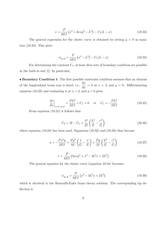
Consider a cantilever beam with rectangular cross-section of unit width. The beam
is loaded by a concentrated force P applied at its tip in the manner shown in Figure 10.1.
c
c
P
y
x
L
1
Figure 10.1: Cantilever Beam Loaded by Concentrated Load
• Elasticity Solution
The elasticity solution for this problem is again obtained using a Airy stress func-
tion [1]. In this case,
Φ = b2xy −
d4
6
xy3
(10.1)
where b2 and d4 are constants. Recalling the relation between stresses in the x−y plane and
Φ, it follows that
σ11 =
∂2
Φ
∂y2
= −d4xy , σ22 =
∂2
Φ
∂x2
= 0 , σ12 = −
∂2
Φ
∂x∂y
= −b2 +
d4
2
y2
(10.2)
The constants b2 and d4 are evaluated by first noting that the longitudinal sides
y = ±c are free from force, implying that σ12 = 0. It therefore follows that
−b2 +
d4
2
y2
= 0 ⇒ b2 =
d4
2
c2
(10.3)
1](https://image.slidesharecdn.com/cantileverelasp-220910092907-ae1debcc/85/cantilever_elas_P-pdf-1-320.jpg)
![10.1 Bending of a Cantilever Loaded at its End
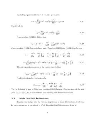
Consider a cantilever beam with rectangular cross-section of unit width. The beam
is loaded by a concentrated force P applied at its tip in the manner shown in Figure 10.1.
c
c
P
y
x
L
1
Figure 10.1: Cantilever Beam Loaded by Concentrated Load
• Elasticity Solution
The elasticity solution for this problem is again obtained using a Airy stress func-
tion [1]. In this case,
Φ = b2xy −
d4
6
xy3
(10.1)
where b2 and d4 are constants. Recalling the relation between stresses in the x−y plane and
Φ, it follows that
σ11 =
∂2
Φ
∂y2
= −d4xy , σ22 =
∂2
Φ
∂x2
= 0 , σ12 = −
∂2
Φ
∂x∂y
= −b2 +
d4
2
y2
(10.2)
The constants b2 and d4 are evaluated by first noting that the longitudinal sides
y = ±c are free from force, implying that σ12 = 0. It therefore follows that
−b2 +
d4
2
y2
= 0 ⇒ b2 =
d4
2
c2
(10.3)
1](https://image.slidesharecdn.com/cantileverelasp-220910092907-ae1debcc/75/cantilever_elas_P-pdf-1-2048.jpg)
![of the beam. Away from the ends (say a distance on the order of the depth of the
beam), Saint-Venant’s principle1
assures that the solution will be satisfactory.
The strains associated with the problem are are related to the stresses through the
constitutive relations. Assuming a linear, isotropic elastic material gives
ε11 =
1
E
(σ11 − νσ22) = −
Pxy
EI
(10.10)
ε22 =
1
E
(σ22 − νσ11) =
νPxy
EI
(10.11)
γ12 =
σ12
G
=
P
2IG
(
y2
− c2
)
(10.12)
The strains are next related to the displacements through the kinematic relations.
Assuming that the displacements and displacement gradients are infinitesimal, it follows
that
ε11 =
∂u
∂x
= −
Pxy
EI
(10.13)
ε22 =
∂v
∂y
=
νPxy
EI
(10.14)
γ12 =
∂u
∂y
+
∂v
∂x
=
P
2GI
(
y2
− c2
)
(10.15)
1
Saint-Venant’s principle states that the stresses some distance from the point of appli-
cation of the load are not affected by the precise behavior of the body close to the point
of application of the load. This principle is named in recognition of the French engineer
and mechanician Adhémar Jean Claude Barré de Saint-Venant (1797-1886). The original
statement of this principle was published in French by Saint-Venant in 1855 [2]. Begin-
ning with the work of von Mises in 1945 [3], the mathematical literature gives a more
rigorous interpretation of Saint-Venant’s principle in the context of partial differential
equations.
3](https://image.slidesharecdn.com/cantileverelasp-220910092907-ae1debcc/85/cantilever_elas_P-pdf-7-320.jpg)
![v =
P
6EI
(
x3
+ 3νxy2
− L3
)
− C1(L − x) (10.33)
The general expression for the elastic curve is obtained by setting y = 0 in equa-
tion (10.33). This gives
v|y=0 =
P
6EI
(
x3
− L3
)
− C1(L − x) (10.34)
For determining the constant C1, at least three sets of boundary condition are possible
at the built-in end [1]. In particular,
• Boundary Condition 1: The first possible constraint condition assumes that an element
of the longitudinal beam axis is fixed; i.e.,
∂v
∂x
= 0 at x = L and y = 0. Differentiating
equation (10.33) and evaluating it at x = L and y = 0 gives
∂v
∂x](https://image.slidesharecdn.com/cantileverelasp-220910092907-ae1debcc/85/cantilever_elas_P-pdf-10-320.jpg)

This document presents the elasticity solution for a cantilever beam with a rectangular cross-section loaded by a concentrated force at its free end. It derives expressions for the stresses, strains, and displacements using the Airy stress function. Three different boundary conditions at the fixed end are considered, resulting in slightly different expressions for the displacements and elastic curve. Shear deformations are found to be more significant for short, deep beams, causing greater transverse deflections than classical beam theory predicts. For beams with span-to-depth ratios over 10, shear effects are negligible and classical theory is accurate.