calipers-and-micrometers.ppt

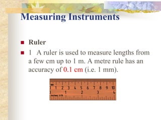
Measuring Instruments
 Ruler
 1 A ruler is used to measure lengths from
a few cm up to 1 m. A metre rule has an
accuracy of 0.1 cm (i.e. 1 mm).

 Ruler
 2 Precautions to be taken when using a ruler:
 (a) Ensure that the object is in contact with the ruler to
avoid inaccurate readings.
 (b) Avoid parallax errors.

 Ruler
 Parallax errors in measurement arise as a result of taking a
reading, with the eye of the observer in the wrong position
with respect to the scale of the ruler. Figure 1.7 shows the
correct position of the eye when reading the scale.
Error = 0.1 cm
Error = 0.1 cm

 Ruler
 (c) Avoid zero and end errors.
 The ends of a ruler, which may be worn out, are a source
of errors in measurement. Thus it is advisable to use the
division mark `1' of the scale as the zero point when
taking a measurement.

 Ruler
 (c) Length of the block, l =3.2cm-1.0cm = 2.2 cm

 1 Lengths
smaller than 1
mm can be
measured with
the help of an
instrument
called a
vernier
caliper.
Vernier Caliper

 Vernier Caliper
 2 A vernier caliper is used to measure an object
with dimensions up to 12 cm with an accuracy of
0.01 cm.

 Vernier Caliper
 3 There are two pairs of
jaws, one is designed to
measure linear dimensions
and external diameters
while the other is to measure
internal diameters.

 Vernier Caliper
 4. To measure with a vernier caliper, slide the vernier
scale along the main scale until the object is held firmly
between the jaws of the caliper. The subsequent steps are
as follows.

 Vernier Caliper
 (a)The reading on the main scale is determined with
reference to the `0' mark on the vernier scale. The reading
to be taken on the main scale is the mark preceding the
Figure 1.10 shows that the '0' mark on the vernier scale
lies between 3.2 cm and 3.3 cm. The reading to be taken
on the main scale is 3.2 cm (the `0' mark on the vernier
scale acts as a pointer).
1

 Vernier Caliper
 (b) The reading to be taken on the vernier scale is indicated by the
mark on the vernier scale which is exactly in line or coincides with
any main scale division line. Figure 1.10 shows that the fourth mark
on the vernier scale is exactly in line with a mark on the main scale.
Thus the second decimal reading of the measurement is:
 Vernier scale reading = 4 x 0.01 cm
 = 0.04 cm
2

 Vernier Caliper

 (c) The reading of the vernier caliper is the result of the
addition of the reading on the main scale to the reading on
the vernier scale.
3.2
0.04

 Vernier Caliper

 (c) The reading of the vernier caliper is the result of the
addition of the reading on the main scale to the reading on
the vernier scale.
 Caliper reading = Main scale Reading + Vernier scale
reading
 Thus the reading of the vernier caliper in Figure 1.10 is
 = 3.2 + 0.04 = 3.24 cm
3.2
0.04

 Vernier Caliper
 5. A vernier caliper has a zero error if the `0'
mark on the main scale is not in line with the '0'
mark on the vernier scale when the jaws of the
caliper are fully closed

 Vernier Caliper
 (a) Positive zero error
 Zero error = +0.04 cm.


0.72 cm
0.70 cm
0.02cm

 Vernier Caliper
(b) Negative zero error
 Zero error = -0.02 cm.

 Micrometer Screw Gauge
1 A micrometer screw gauge is used to measure
small lengths ranging between 0.10 mm and
25.00 mm.

2 This instrument can be used to measure diameters
of wires and thicknesses of steel plates to an
accuracy of 0.01 mm.

3 The micrometer scale comprises a main scale marked on
the sleeve and a scale marked on the thimble called the
thimble scale.

4 The difference between one division on the upper scale
and one division on the lower scale is 0.5 mm.

Micrometer Screw Gauge
5 The thimble scale is subdivided into 50 equal divisions.
When the thimble is rotated through one complete turn, i.e.
360, the gap between the anvil and the spindle increases
by 0.50 mm.

6 This means that one division on the thimble scale
is = 0.01 mm.
50
5
.
0 mm

7 When taking a reading, the thimble is turned until
the object is gripped very gently between the
anvil and the spindle.

8 The ratchet knob is then turned until a `click'
sound is heard.

9 The ratchet knob is used to prevent the user
from exerting undue pressure.

10 The grip on the object must not be excessive as
this will affect the accuracy of the reading.

11 Readings on the micrometer are taken as follows.
(a) The last graduation showing on the main scale
indicates position between 2.0 mm and 2.5 mm.
Thus the reading on the main scale is read as 2.0
mm.

(b) The reading of the micrometer screw gauge is the
sun of the main scale reading and the thimble
scale reading which is:
 2.0 + 0.22 =2.22 mm

(b) The reading on the thimble scale is the point
where the horizontal reference line of the main
scale is in line with the graduation mark on the
thimble scale Figure 1.15(b) shows this to be the
22nd mark on the thimble scale, thus giving a
reading of 22 x 0.01 mm = 0.22 mm.

(a) Positive zero error
 In Figure 1.16, the horizontal reference line in the main
scale is in line with the 4th division mark, on the positive
side of the `0' mark, on the thimble scale. The error of
+0.04 mm must be subtracted from all readings taken.
 Zero error = +0.04 mm

13(b) Negative zero error
In Figure 1.17, the horizontal reference line on
the main scale is in line with the 3rd division mark,
below the `0' mark of the thimble scale.
Zero error = -0.03 mm

Chapter 1
1.5 ANALYSING SCIENTIFIC
INVESTIGATION

INVESTIGATION
 1. The investigative procedure begins with the following
steps:

 Making an inference
 To interpret or explain what is being observed. It is also
an early conclusion based on observation.

INVESTIGATION
 Determining the variables
 A variable is a physical quantity which varies/changes
during the course of a scientific investigation.

INVESTIGATION
 In a scientific investigation, there are 3 different types of
variables, namely:
 (a) Manipulated variable
 • It is a physical quantity which is fixed in an
experiment.
 (b) Responding variable
 • It is a physical quantity which depends on the
independent variable.
 (c) Constant variable
 • It is a physical quantity which is fixed while an
experiment is being carried out.

INVESTIGATION
 Making a hypothesis
 It is a clarification/explanation regarding the
relationship between the manipulated variable
and the responding variable when all other
variables are kept constant.

 A hypothesis must be proven correct after an
experiment is carried out.

INVESTIGATION
 Controlling the variable
 The experiment must be conducted in an
appropriate place so as not to influence the
variables.

INVESTIGATION
 Planning the investigative procedure/method
 Covers the choice and arrangement of the
apparatus together with the work procedure being
followed/ conducted.

INVESTIGATION
 Collecting data in tabular form
 Data in the same strips (i.e., rows and columns)
must have the same units and the same number of
decimal places (ie., data must be consistent).

 For example:

INVESTIGATION
 1. The investigative procedure begins with
the following steps:

 Collecting data in tabular form
 For example:

INVESTIGATION
 Interpreting the data
 It is a result/decision that is made by way
of the experiment.

INVESTIGATION
 Making a conclusion
 It is a record that is made regarding an
information that is being studied based on the aim
of the experiment.
 The conclusion which is made is based on the
shape of the graph that is plotted and also on the
value(s) of the quantities obtained through
calculation using a formula.

INVESTIGATION
 Making a complete report of an experiment
 A complete report of an experiment must cover
all the following aspects:
 • Problem statement
 • Inference
 • Hypothesis
 • Aim of experiment
 • Variables of the experiment
 • Arrangement of apparatus/Materials used

INVESTIGATION
 Making a complete report of an experiment
 • Experimental procedure - including the method for
controlling the manipulated and responding variables.
 • Tabulating data
 • Analyzing data
 • Making a conclusion
 • Data tabulation
 • Data analysis

INVESTIGATION
 Experiment 1.1
 To Study The Relationship Between The Length
Of A Pendulum And The Period Of Oscillation of
The Pendulum

 Problem Statement
 How can the period of oscillation of a pendulum
be determined?


INVESTIGATION
 Experiment 1.1
 To Study The Relationship Between The Length Of A
Pendulum And The Period Of Oscillation of The
Pendulum

 Hypothesis
 As the length of the pendulum increases, its period of
oscillation increases.


INVESTIGATION
 Variables
 (a) Manipulated : Length of pendulum
 (b) Responding : Period of oscillation
 (c) Constant: Amplitude of oscillation, mass of pendulum
bob (or weight) and acceleration due to gravity.

INVESTIGATION
 Experiment 1.1
 Apparatus/Materials Used
 Pendulum bob, a 100cm length of thread, metre rule, 2
small pieces of wood, retort stand and a stop-watch.


INVESTIGATION
 Experiment 1.1
 To Study The Relationship Between The Length Of A
Pendulum And The Period Of Oscillation of The
Pendulum
 Procedure

INVESTIGATION
 Experiment 1.1
 To Study The Relationship Between The Length Of A Pendulum And
The Period Of Oscillation of The Pendulum

 Procedure
 1. A 50.0g pendulum bob is tied to one end of a 100cm length
thread.
 2. By using a retort stand and two small pieces of wood, the other
end of the thread is clamped as shown in Diagram 1.19.
 3. The length, l of the pendulum is measured from the end below
the small piece of wood to the centre of the bob. (i.e., l = 20cm)
 4. The pendulum is made to oscillate in a plane and having a small
amplitude of oscillation. (i.e., approximately 10°)

INVESTIGATION
Procedure
 5. The time taken to complete 20 full oscillations is recorded with a
stop-watch.
 6. The time for 20 complete oscillations is recorded once more.
 7. The average time taken in the above two steps is calculated, so
too with the time taken.
 8. The experimental procedure is repeated by taking the length of
the pendulum to be l = 30cm, 40cm, 50cm, 60 cm and 70cm.
 9. All readings obtained are recorded in a table.
 10. Then, a graph of T against l is plotted.

INVESTIGATION
 Result:


INVESTIGATION
 Graph T against L:

INVESTIGATION
 Experiment 1.1
 Discussion:
 Graph of period, T against length, L shows a curve with
positive gradient. Thus, as L increases, T also increases.
Hence, the hypothesis is accepted.

INVESTIGATION
 Conclusion:
 The longer is the length of the pendulum, the longer is the
period of its oscillation.

calipers-and-micrometers.ppt

Recommended

Recommended

More Related Content

Similar to calipers-and-micrometers.ppt

Similar to calipers-and-micrometers.ppt (20)

Recently uploaded

Recently uploaded (20)

calipers-and-micrometers.ppt