Downloaded 16 times

![DATA DESCRIPTION
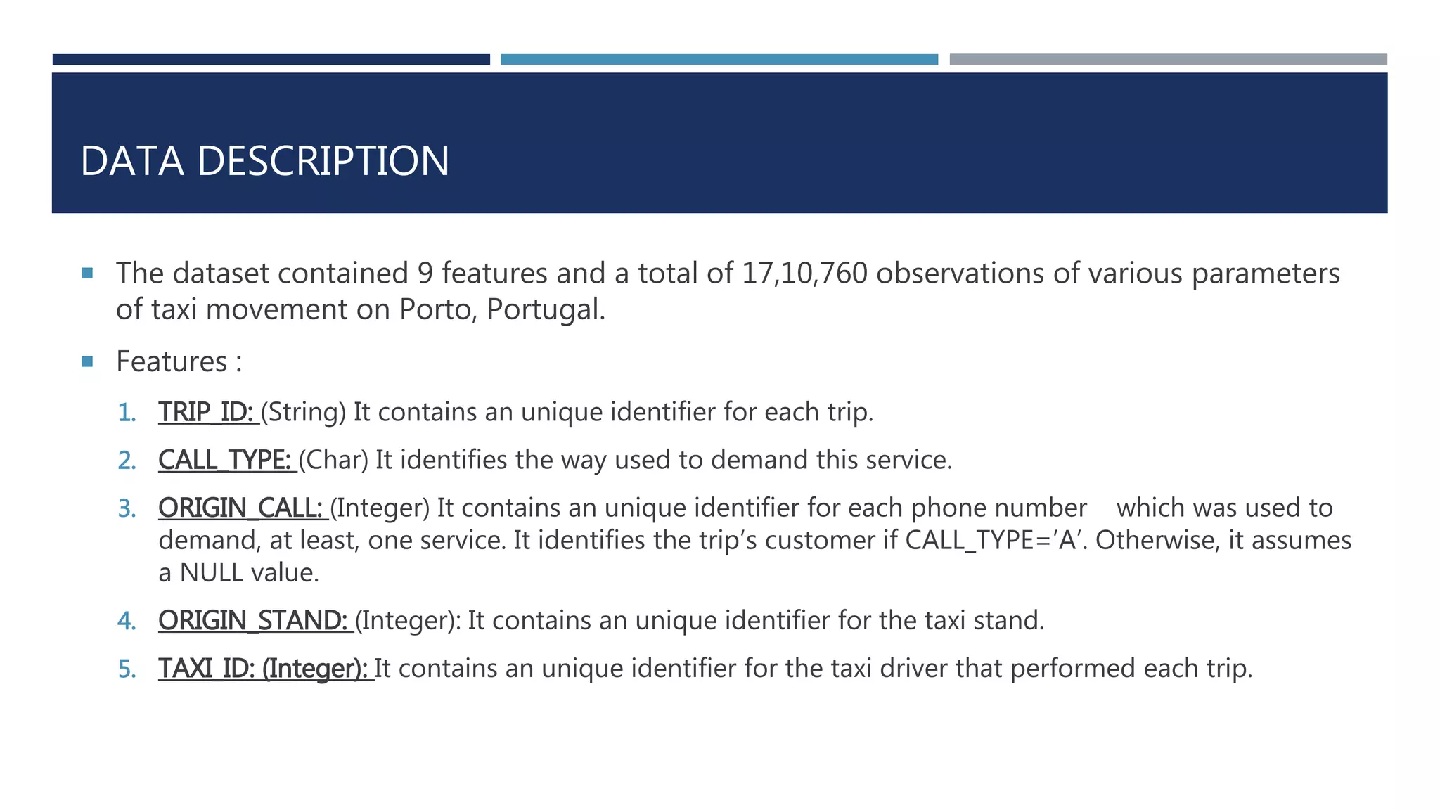
The dataset contained 9 features and a total of 17,10,760 observations of various parameters
of taxi movement on Porto, Portugal.
Features :
6. TIMESTAMP: (Integer) Unix Timestamp (in seconds). It identifies the trip’s start.
7. DAYTYPE: (Char) It identifies the type of the day in which the trip starts. (Holiday, Day before Holiday,
Weekday)
8. MISSING_DATA: (Boolean) It is FALSE when the GPS data stream is complete and TRUE whenever one
(or more) locations are missing.
9. POLYLINE: (String): It contains a list of GPS coordinates (i.e. WGS84 format) mapped as a string. Each
pair of coordinates is of the form [LONGITUDE, LATITUDE].
For Prediction of Time we have considered Timestamp and Polyline.
The rows having missing value are not considered in our calculations.](https://image.slidesharecdn.com/cabtraveltimeprediction-160310225900/75/Cab-travel-time-prediction-using-ensemble-models-5-2048.jpg)
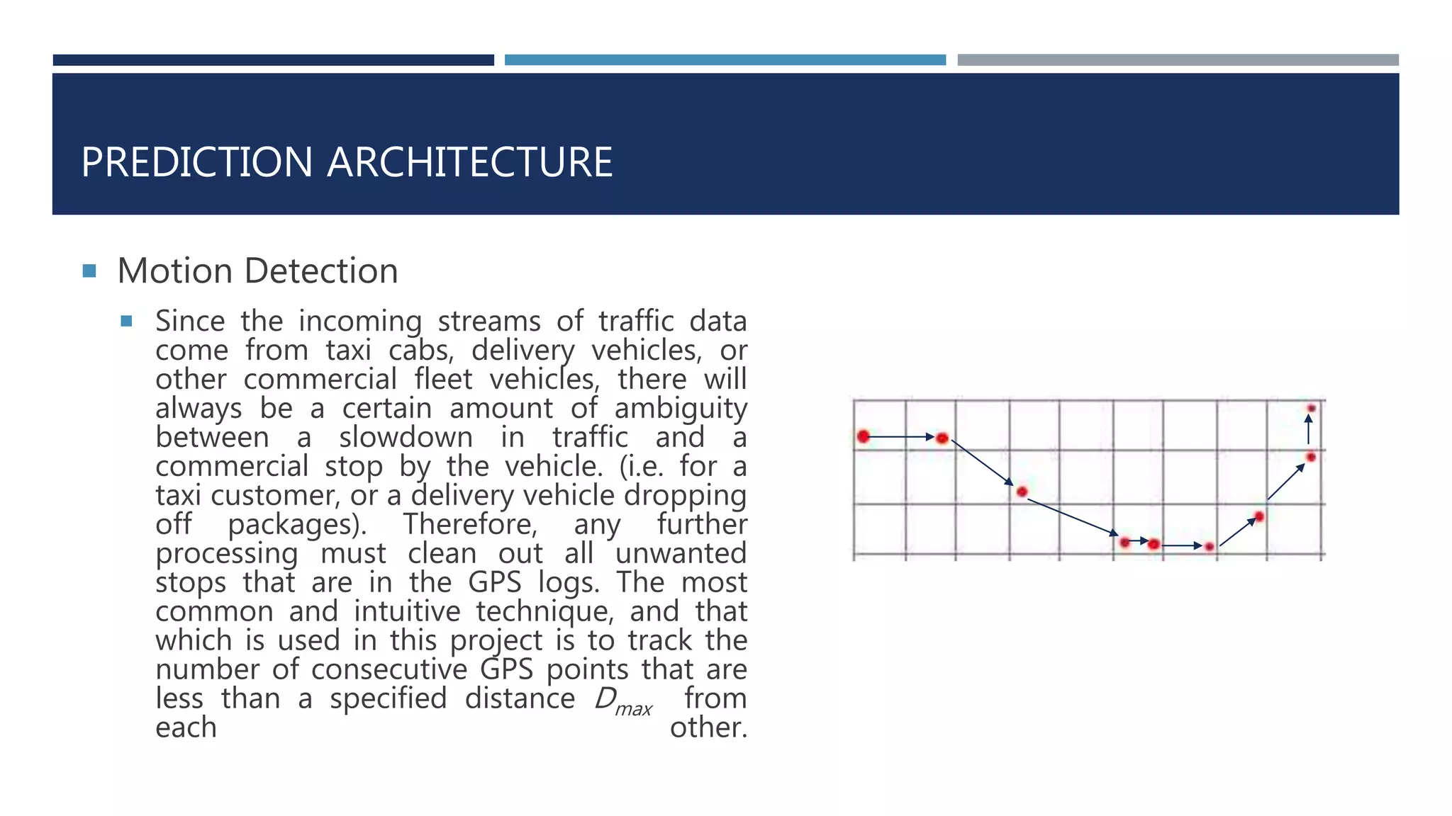

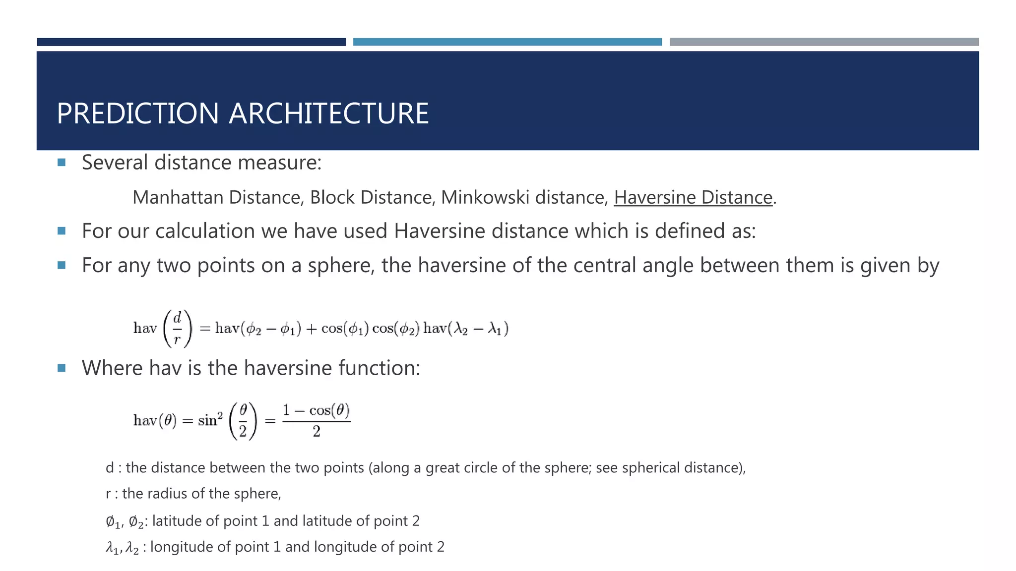
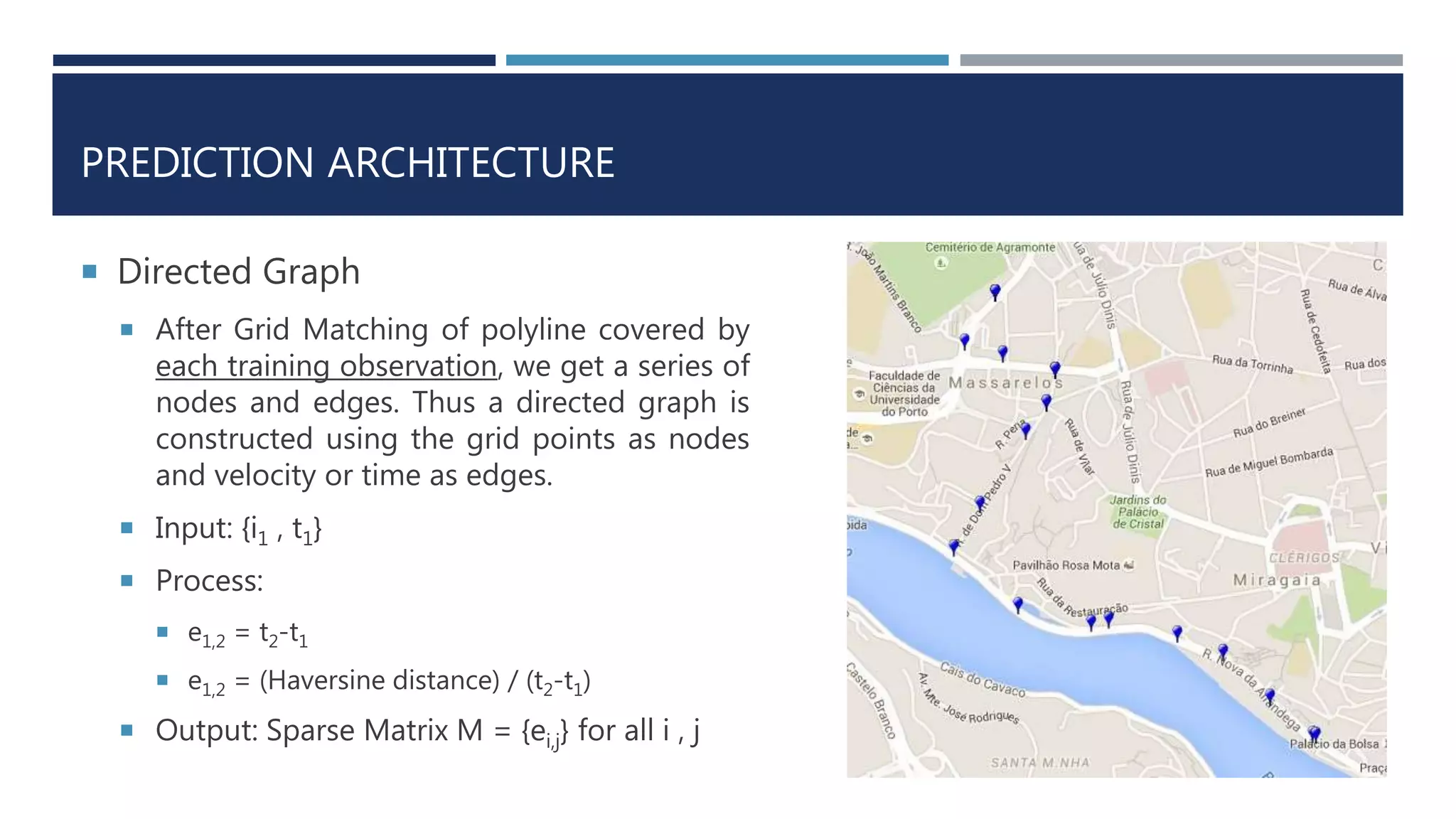
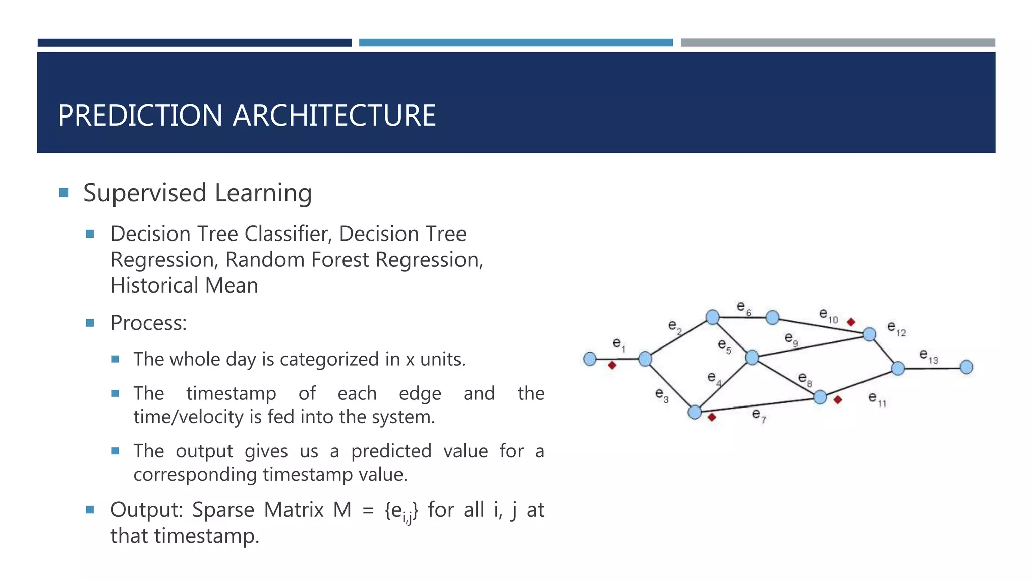
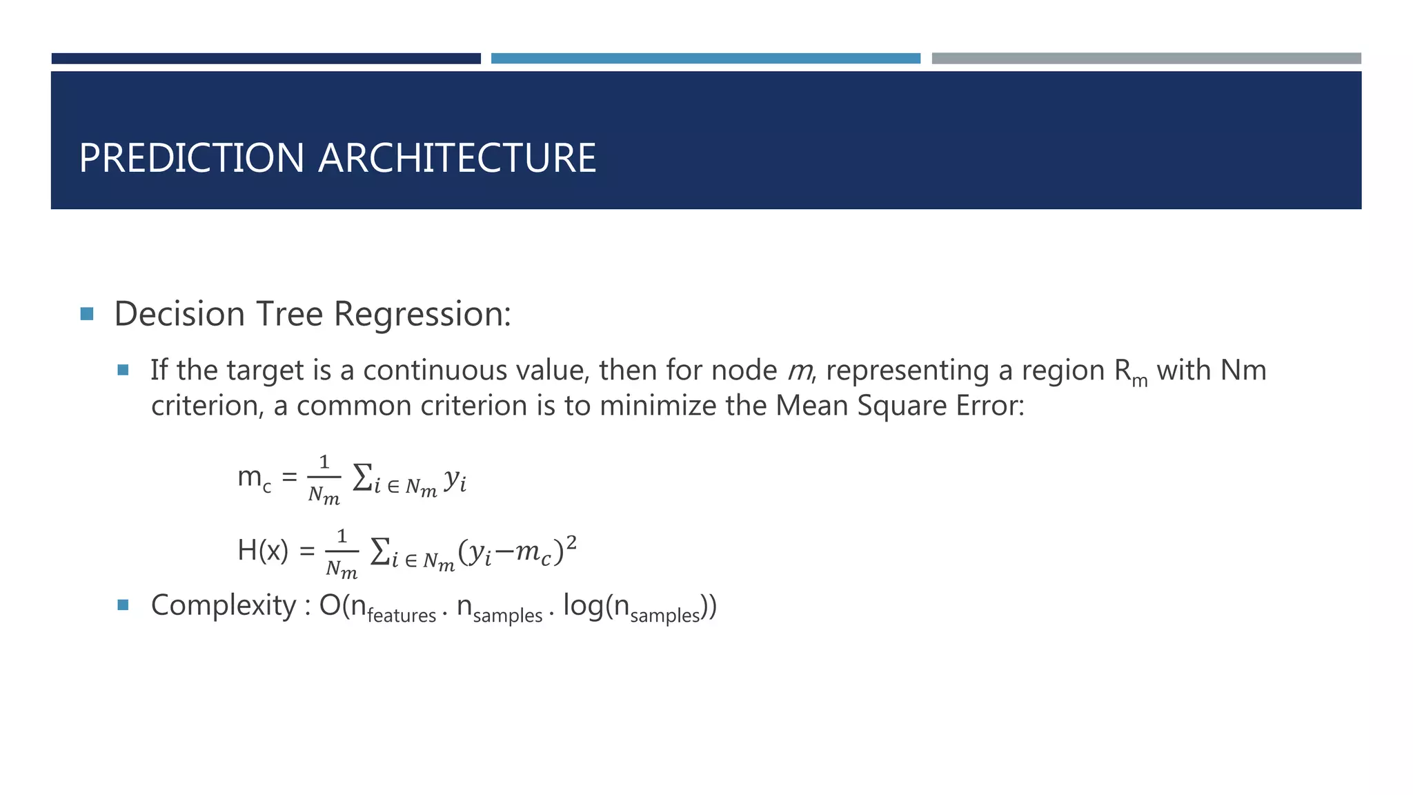
![PREDICTION ARCHITECTURE
Decision Tree Classification:
Classification trees work just like regression trees, only they try to predict a discrete
category (the class), rather than a numerical value. The response variable Y is categorical,
so we can use information theory to measure how much we learn about it from knowing
the value of another discrete variable A:
I[Y | A] = 𝑎 P A = a ∗ I[Y | A = a]
Where, I[Y | A = a] = H[Y ] − H[Y | A = a]
The definitions of entropy H[Y ] and conditional entropy H[Y |A = a].
H[Y | A = a] = - 𝑘 𝑝 𝑎𝑘 log2 𝑝 𝑎𝑘](https://image.slidesharecdn.com/cabtraveltimeprediction-160310225900/75/Cab-travel-time-prediction-using-ensemble-models-12-2048.jpg)
![DATA INFERENCE
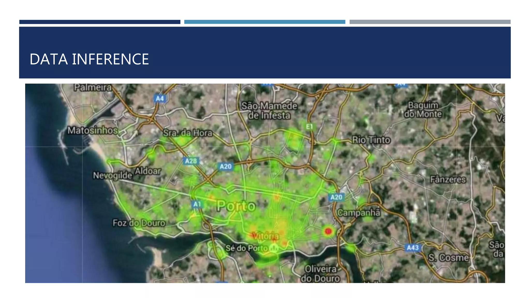
Top 5 important road segments of the city are
[[41.162292, -8.60787], [41.162031, -8.60571]]
[[41.16258, -8.61003], [41.162292, -8.60787]]
[[41.163291, -8.6157], [41.163021, -8.613639]]
[[41.163525, -8.617644], [41.163291, -8.6157]]
[[41.163768, -8.619678], [41.163525, -8.617644]]
0.0772321809805613, 0.07708869873451546, 0.07441287173742973, 0.07212227668575326,
0.06932519386480848
Rank Segment Centrality
1 [41.162292, -8.60787], [41.162031, -
8.60571]
0.0772321809805613
2 [41.16258, -8.61003], [41.162292, -8.60787] 0.0770886987345154
6
3 [41.163291, -8.6157], [41.163021, -
8.613639]
0.0744128717374297
3
4 [41.163525, -8.617644], [41.163291, -
8.6157]
0.0721222766857532
6](https://image.slidesharecdn.com/cabtraveltimeprediction-160310225900/75/Cab-travel-time-prediction-using-ensemble-models-20-2048.jpg)
![DATA INFERENCE
Rank Geo-Location Centrality
1 [41.162031, -8.60571] 0.08277015940786502
2 [41.162292, -8.60787] 0.07877967724696255
3 [41.16258, -8.61003] 0.07775467831692078
4 [41.163021, -
8.613639]
0.07690847152899795
5 [41.163291, -8.6157] 0.07608514260606453](https://image.slidesharecdn.com/cabtraveltimeprediction-160310225900/75/Cab-travel-time-prediction-using-ensemble-models-21-2048.jpg)
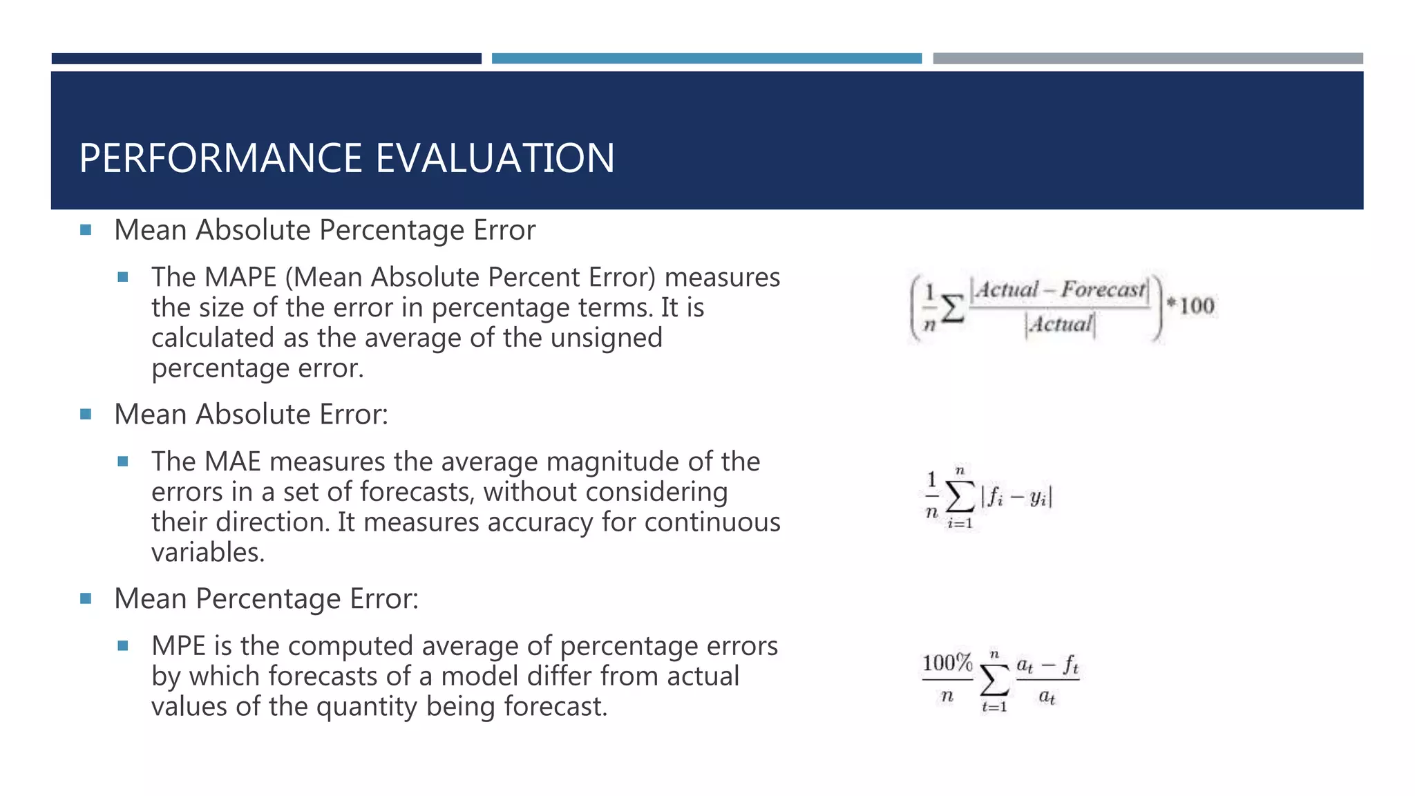
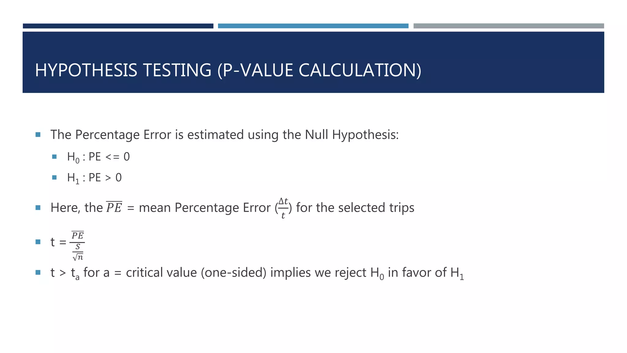
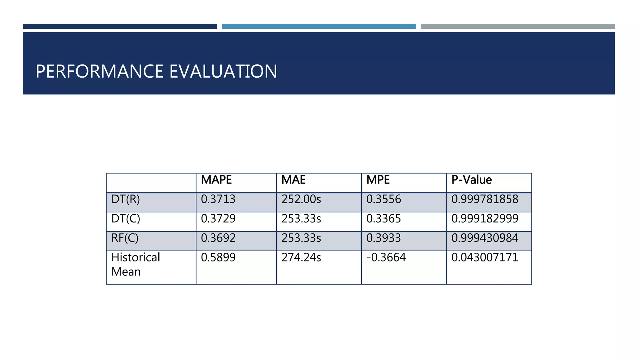
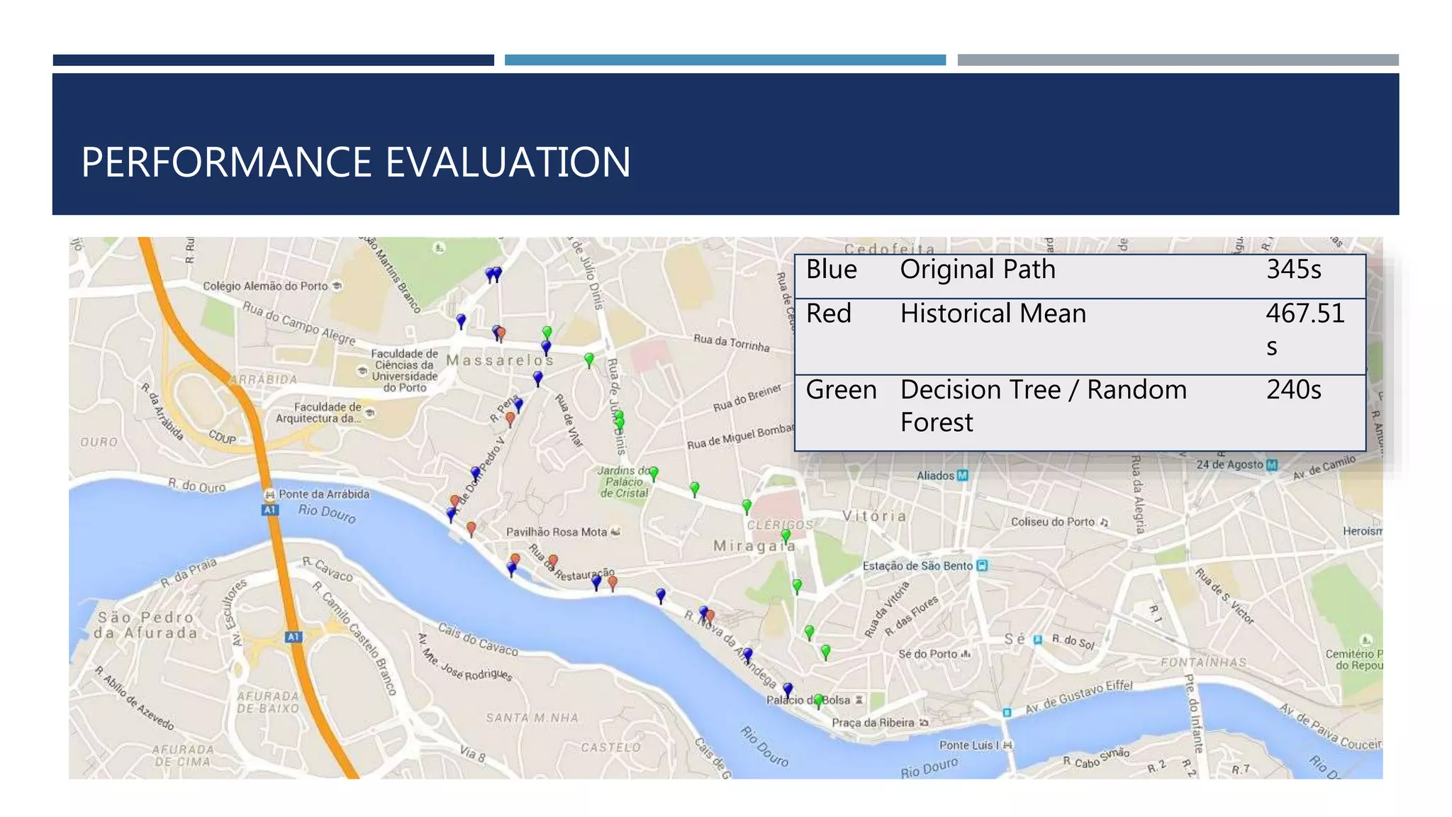
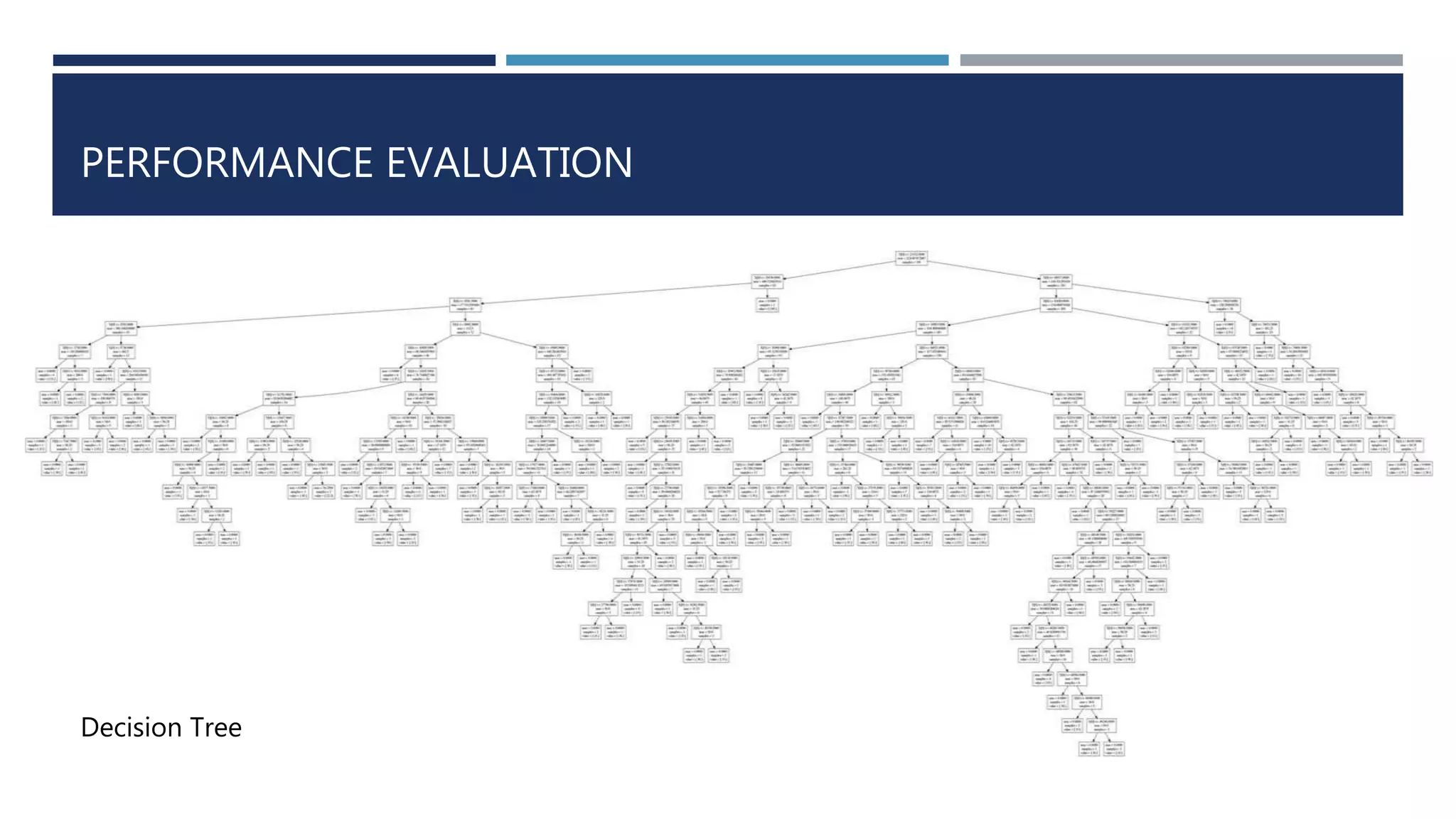


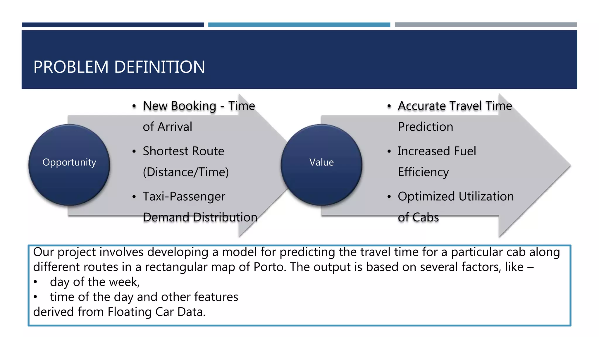
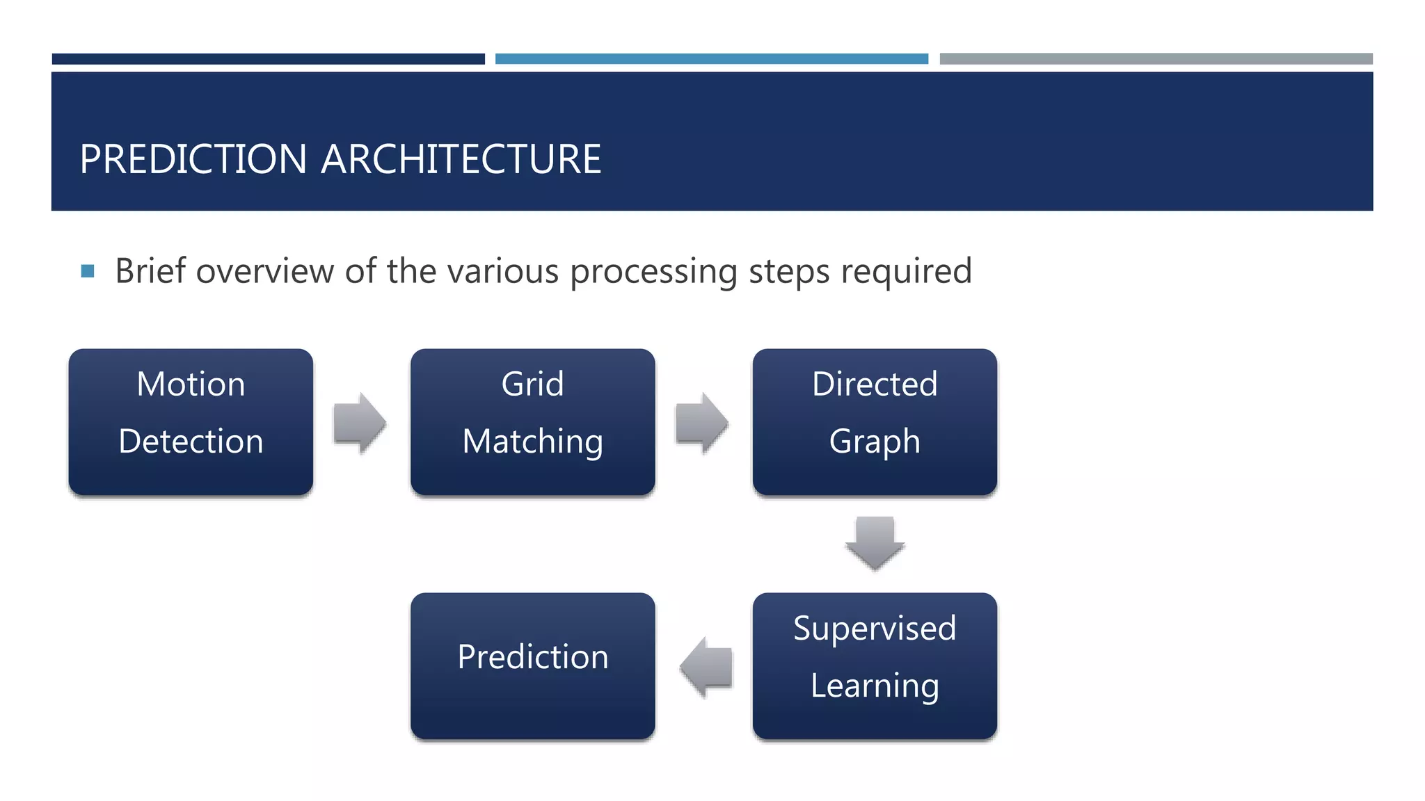
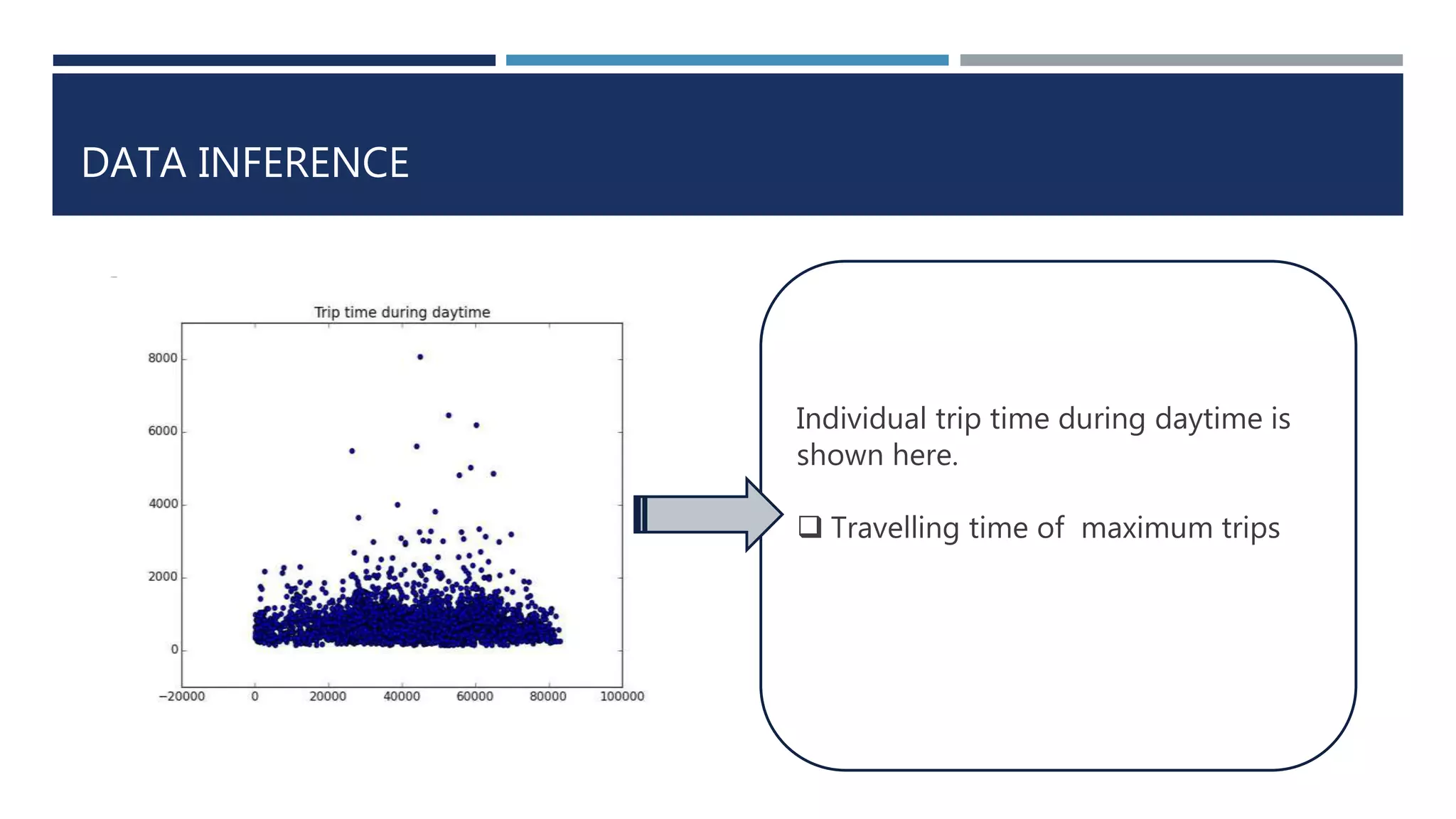
This document discusses developing a model to predict taxi travel times along different routes in Porto, Portugal based on floating car data. It involves motion detection on GPS data to identify stops, grid matching to map GPS coordinates to a road network, building a directed graph of the network, and using supervised learning methods like decision trees on historical travel times to predict times for new trips. Key factors in the predictions are day of week, time of day, and features derived from taxi GPS data. The model performance is evaluated based on mean absolute percentage error, mean absolute error, and mean percentage error.


![[DSC Europe 25] Vid Stimac - Policy Parsimony: Between Oversimplifying and Ov...](https://cdn.slidesharecdn.com/ss_thumbnails/eqlepagzqp2rhg3gbluh-dsc-stimac-251120-251205090438-059e7f54-thumbnail.jpg?width=640&height=640&fit=bounds)
![[DSC Europe 25] Max Talanov - Non digital NNs.pptx](https://cdn.slidesharecdn.com/ss_thumbnails/wif8tr3gtua74qvtopke-non-digital-nns-251205090438-26b0eea6-thumbnail.jpg?width=640&height=640&fit=bounds)
![[DSC Europe 25] Marija Vlajkovic & Andrea Radonjanin - Integration of AI tool...](https://cdn.slidesharecdn.com/ss_thumbnails/qf1jrglttoc3bm8s3aop-final-integration-of-ai-tools-251208151905-394f3a6a-thumbnail.jpg?width=640&height=640&fit=bounds)
![[DSC Europe 25] Jim Sterne - Adopting Generative AI Capabilities Into the Ent...](https://cdn.slidesharecdn.com/ss_thumbnails/sxhpofuorcagxsaulkmt-3-251204082258-7e66bc48-thumbnail.jpg?width=640&height=640&fit=bounds)


![[DSC Europe 25] Dragan Vucic - Building the Learning Organization - How AI Tr...](https://cdn.slidesharecdn.com/ss_thumbnails/8brigo2sbu6qur6gxrra-7-251205085715-6ae07d24-thumbnail.jpg?width=640&height=640&fit=bounds)
![[DSC Europe 25] Petar Zivanov - AI meets documents From chatbots to AI-powere...](https://cdn.slidesharecdn.com/ss_thumbnails/xer2bb6nrdc8pdpev0pc-8-251204082258-7c2fa4a1-thumbnail.jpg?width=640&height=640&fit=bounds)
