The document presents a complete Android-based framework for automatically identifying a user's transportation mode using GPS trajectories and accelerometer measurements from a smartphone. The framework includes an architecture, design, implementation, user interface, and algorithms for transportation mode identification. It applies segmentation, simplification, and machine learning classification techniques to collected GPS and accelerometer data to identify modes like walking, running, and in-vehicle transportation. The system was evaluated on real and simulated data, achieving an overall accuracy of around 85% for identifying transportation modes, outperforming the Google Activity Recognition API.

1. Complete Framework for Automatic
Transportation Mode Identification
Kotsomitopoulos Aristotelis
TH
E
U
N I V E R
S
ITY
OF
E
D I N B U
R
G
H
Master of Science
Computer Science
School of Informatics
University of Edinburgh
2016

3. Abstract
Transportation mode identification techniques using smartphones or sensors can help
in transportation research and especially in traffic planning. We present a complete
Android based framework system including an architecture, design, implementation
and user interface. We demonstrate some of the most used systems and techniques to
infer activities along with their accuracy. The primary contributions of our work is to
create an android application with the ability to automatically identify the users trans-
portation mode (walking, running, in vehicle) using GPS trajectories and accelerome-
ter measurements. To achieve this we apply multiple segmentation, simplification and
machine learning classification techniques on our collected data sets. We also used
some approaches to improve our systems efficiency, responsiveness and battery con-
sumption. We present the results to the user in a smooth and user friendly way, while
we demonstrate some interesting facts like the travel distance and the speed in order
to make our application more attractive. We evaluated the accuracy of our algorithms
using both manually collected data as well as the Geolife public dataset. We compared
it with popular ML classification techniques and the Google API for activity recogni-
tion. We observed that our algorithms work more accurate than the Google API and
we achieved quite impressive results with an overall accuracy of about 85%.
iii

4. Acknowledgements
I would like to express my deepest sens of gratitude to my supervisor Rik Sarkar for
his continuous support through this project. His guidance helped me in all the time of
research and writing of this thesis.
I thank my friends for the stimulating discussions and for the sleepless nights we were
working and supporting each other.
Last but not the least, I would also like to thank my parents and my brother for sup-
porting me spiritually throughout writing this thesis and my life in general.
iv

5. Declaration
I declare that this thesis was composed by myself, that the work contained herein is
my own except where explicitly stated otherwise in the text, and that this work has not
been submitted for any other degree or professional qualification except as specified.
(Kotsomitopoulos Aristotelis)
v

7. Table of Contents
1 Introduction 1
1.1 Purpose of the Thesis . . . . . . . . . . . . . . . . . . . . . . . . . . 1
1.2 Motivation of the Thesis . . . . . . . . . . . . . . . . . . . . . . . . 2
1.3 Challenges of the Thesis . . . . . . . . . . . . . . . . . . . . . . . . 2
1.4 Structure of the Thesis . . . . . . . . . . . . . . . . . . . . . . . . . 3
1.5 Outcome of the Thesis . . . . . . . . . . . . . . . . . . . . . . . . . 3
2 Background 5
2.1 Sensors Used in the Literature . . . . . . . . . . . . . . . . . . . . . 5
2.1.1 Global Positioning System (GPS) . . . . . . . . . . . . . . . 5
2.1.2 Accelerometer . . . . . . . . . . . . . . . . . . . . . . . . . 6
2.1.3 Wireless Fidelity-Wireless Internet (Wi-Fi) . . . . . . . . . . 6
2.1.4 Global System for Mobile Communications (GSM) . . . . . . 6
2.2 Related Work . . . . . . . . . . . . . . . . . . . . . . . . . . . . . . 7
2.2.1 First Steps . . . . . . . . . . . . . . . . . . . . . . . . . . . 7
2.2.2 Sensor-Based Transportation Mode Identification . . . . . . . 8
2.2.3 Wi-Fi and GSM . . . . . . . . . . . . . . . . . . . . . . . . . 10
2.2.4 GPS and Accelerometer . . . . . . . . . . . . . . . . . . . . 10
2.3 Useful Algorithms . . . . . . . . . . . . . . . . . . . . . . . . . . . 11
2.3.1 Radial Distance . . . . . . . . . . . . . . . . . . . . . . . . . 11
2.3.2 Douglas-Peucker . . . . . . . . . . . . . . . . . . . . . . . . 12
3 Design and Functionality 15
3.1 Tools and Technologies Used . . . . . . . . . . . . . . . . . . . . . . 15
3.1.1 Android Development . . . . . . . . . . . . . . . . . . . . . 16
3.1.2 External Tools . . . . . . . . . . . . . . . . . . . . . . . . . 16
3.2 Architecture and Functionality . . . . . . . . . . . . . . . . . . . . . 17
vii

8. 3.2.1 Main Application Thread . . . . . . . . . . . . . . . . . . . . 18
3.2.2 Background Tracking Activity . . . . . . . . . . . . . . . . . 18
3.2.3 Background Service . . . . . . . . . . . . . . . . . . . . . . 20
3.2.4 View Recordings . . . . . . . . . . . . . . . . . . . . . . . . 21
3.2.5 View Statistics . . . . . . . . . . . . . . . . . . . . . . . . . 23
3.2.6 Database . . . . . . . . . . . . . . . . . . . . . . . . . . . . 25
4 Implementation and Development 27
4.1 Transportation Mode Identification . . . . . . . . . . . . . . . . . . . 27
4.1.1 GPS Error Handling . . . . . . . . . . . . . . . . . . . . . . 27
4.1.2 Extracting Values . . . . . . . . . . . . . . . . . . . . . . . . 29
4.1.3 Segmentation using GPS . . . . . . . . . . . . . . . . . . . . 31
4.1.4 Walking vs Running . . . . . . . . . . . . . . . . . . . . . . 35
4.1.5 Identification . . . . . . . . . . . . . . . . . . . . . . . . . . 36
4.1.6 Classification . . . . . . . . . . . . . . . . . . . . . . . . . . 38
4.1.7 Dataset Creation . . . . . . . . . . . . . . . . . . . . . . . . 38
4.1.8 Create and Exporting Models . . . . . . . . . . . . . . . . . 39
4.1.9 Using The Model . . . . . . . . . . . . . . . . . . . . . . . . 40
4.2 Processes and Communication . . . . . . . . . . . . . . . . . . . . . 40
4.2.1 Foreground Service . . . . . . . . . . . . . . . . . . . . . . . 41
4.2.2 View Recording . . . . . . . . . . . . . . . . . . . . . . . . . 42
4.3 Reducing Battery Consumption . . . . . . . . . . . . . . . . . . . . . 43
4.4 User Interface . . . . . . . . . . . . . . . . . . . . . . . . . . . . . . 44
5 Evaluation 47
5.1 Parameter Selection . . . . . . . . . . . . . . . . . . . . . . . . . . . 47
5.2 Accuracy and Tests Using Segmentation . . . . . . . . . . . . . . . . 48
5.2.1 Real Life . . . . . . . . . . . . . . . . . . . . . . . . . . . . 48
5.2.2 Simulation . . . . . . . . . . . . . . . . . . . . . . . . . . . 50
5.3 Classification . . . . . . . . . . . . . . . . . . . . . . . . . . . . . . 51
5.4 Comparison with Google API . . . . . . . . . . . . . . . . . . . . . 52
5.5 Battery Consumption . . . . . . . . . . . . . . . . . . . . . . . . . . 53
6 Conclusion and Future Work 55
Bibliography 57
viii

9. List of Figures
2.1 Accelerometer readings from different activities . . . . . . . . . . . . 11
3.1 System Architecture . . . . . . . . . . . . . . . . . . . . . . . . . . . 17
3.2 main menu and tracking screenshots . . . . . . . . . . . . . . . . . . 19
3.3 Custom notification bar . . . . . . . . . . . . . . . . . . . . . . . . . 21
3.4 Transportation mode identification final results . . . . . . . . . . . . 22
3.5 Recordings and chart screenshots . . . . . . . . . . . . . . . . . . . . 23
3.6 Past month results representation . . . . . . . . . . . . . . . . . . . . 24
3.7 Relational database design scheme . . . . . . . . . . . . . . . . . . . 25
4.1 Inaccurate points . . . . . . . . . . . . . . . . . . . . . . . . . . . . 27
4.2 Before and after smoothing velocity . . . . . . . . . . . . . . . . . . 29
4.3 Trajectory sequence sample . . . . . . . . . . . . . . . . . . . . . . . 33
4.4 Trajectory sequence after the first stage . . . . . . . . . . . . . . . . 33
4.5 Trajectory sequence after the second stage . . . . . . . . . . . . . . . 33
4.6 Bus segment interpolated by walking segments . . . . . . . . . . . . 35
4.7 Accelerometer measurements for walking and running . . . . . . . . 36
4.8 Filtering the segmentation list using accelerometer measurements . . 37
4.9 Function for filtering running and notRunning points . . . . . . . . . 37
4.10 Retrieving the stored data from database . . . . . . . . . . . . . . . . 43
4.11 Description on long press click for clarity . . . . . . . . . . . . . . . 44
4.12 Correlation between colors and transportation modes . . . . . . . . . 46
5.1 11 km of pure walking achieved 99.9% accuracy . . . . . . . . . . . 48
5.2 2 km of pure running achieved 99% accuracy . . . . . . . . . . . . . 49
5.3 10km on a bus with some traffic achieved 81% accuracy . . . . . . . 50
5.4 Segmentation results from Geolife trajectory (19170 points) . . . . . 51
5.5 Function for filtering in vehicle points according to Google API . . . 52
ix

10. 5.6 Our approach versus Google API . . . . . . . . . . . . . . . . . . . . 53
5.7 Battery consumption . . . . . . . . . . . . . . . . . . . . . . . . . . 54
x

11. Chapter 1
Introduction
Undoubtedly, mobile devices are the most used technological devices all over the
world. Smartphones are becoming the most dominant device to be seen since the
mobiles inception. According to latest research, there are more than two billion smart-
phone users while the number is expected to be increased by 12% next year12. The
majority of those smartphones are equipped with various sensors and features. Due to
all those new features the transportation mode identification is now feasible from al-
most every smartphone device. During the past years, a lot of GPS based systems have
succeed to identify the users transportation mode. However, the majority of the GPS
trajectories contain various errors and especially in slow speed activities like walking.
This is why we will use one more sensor in our implementation to improve the accu-
racy, the accelerometer. The accelerometer is able to measure the acceleration of the
handset along the three axes (x,y and z) multiple times per second.
1.1 Purpose of the Thesis
The aim of this project is, by taking advantage of all those new features, to create an
appealing android application that has the ability to automatically identify the trans-
portation mode and the activity of the user (walking, running, on vehicle). We will
not only create an android application but also we will create a complete framework
from scratch including (design and architecture, relational databases, threads and ser-
vices, algorithms and the main business logic for identification, User Interface). We
will focus our research on retrieving and analyzing data from GPS trajectories and
1http://thehub.smsglobal.com/smartphone-ownership-usage-and-penetration
2http://www.emarketer.com/Article/2-Billion-Consumers-Worldwide-Smartphones-by-
2016/1011694
1

12. 2 Chapter 1. Introduction
accelerometer measurements in order to apply multiple algorithms and techniques on
them like segmentation, simplification and classification. We will also try to improve
and compare our results with other popular Machine Learning classification methods.
Furthermore, we will compare our experiments with the latest feature of the Google
API about human activity recognition. Finally, we will try to reduce the battery con-
sumption while GPS and Accelerometer have an increased power consumption. We
combined all those different approaches and we achieved improved results regarding
the accuracy, validity and efficiency.
1.2 Motivation of the Thesis
Information about the transportation mode can be useful for multiple applications.
Public transportation companies can take advantage of this data to predict and avoid
traffic jams, while they can also organize better the vehicle routes and the number of the
required transportation means in each place. Efficient and faster daily transportation
can lead to a much better lifestyle. In addition, mobile applications can change their
behavior according to the users activity. For instance, with real time transportation
mode identification, companies may block the use of some applications while driving
for safety reasons. Athletes and runners can also take advantage of tose features to
track themselves between different activities. Through the past few years, multiple ap-
proaches have been made using and trying a lot of different technologies, sensors and
techniques all for the same motive, to improve the accuracy. The more accurate the
results the greater the benefit.
1.3 Challenges of the Thesis
There are several problems we have to overcome in order to achieve notable results.
The main problem is that even the latest GPS technology has multiple measurement er-
rors and signal losses so we have to minimize them. The next challenge is the way we
will analyze our data (the main algorithmic logic of our application) and the techniques
we will apply (classification and segmentation) to accurately identify the transporta-
tion mode. In addition to that, we have to properly merge the data from all the different
kind of measurements in order to achieve a solid data set. Subsequently, there is the
difficulty of retrieving and storing the required data in a relational database concur-
rently by taking full advantage of the hardware resources like multi-core processors

13. 1.4. Structure of the Thesis 3
and threading. Finally, the last problem is to find a way to demonstrate the results and
appeal the users to use the application, otherwise not enough data would be collected
for sufficient results. These problems, have motivated our research in order to develop
efficient and improved algorithms to overcome them.
1.4 Structure of the Thesis
The current thesis is structured as follows. In Chapter 2 we set the appropriate back-
ground, relative works and the exposition of relevant literature. In Chapter 3 we
demonstrate the technologies we used, our system architecture and design as well as
the detailed functionality of every component. Then, in Chapter 4 we describe our
implementation and development process. In Chapter 5 we evaluate our methods and
we compare them with other popular approaches. Finally, in Chapter 6 we present the
limitation of our work and we suggest possible enhancements.
1.5 Outcome of the Thesis
We used manually collected data as well as the Geolife public dataset for our evalu-
ation. The results we observed using our segmentation algorithms are quite impres-
sive with an overall accuracy of 85% while for identifying Walking and Running we
achieved an accuracy of 95%. The Classification using decision trees approach was a
bit less accurate with an accuracy of about 83%. We also concluded that our implemen-
tation has an even better accuracy than the current Google API for activity recognition.
The application tested in multiple mobile phones and emulators, it works and runs
smoothly without any crashes.

15. Chapter 2
Background
This chapter explains and demonstrates the technical background that is relevant to this
project. It also contains an explanation of the main smartphones sensors that will help
us with the transportation mode identification. The relative work and algorithms that
have been done using some of those sensors.
2.1 Sensors Used in the Literature
In this section we will briefly describe the way some of the most commonly used
sensors (GPS, WiFi, GSM and Accelerometer) work. They are all available in almost
every new mobile device.
2.1.1 Global Positioning System (GPS)
Global Positioning System (GPS) is a navigation system that provides location any-
where on earth along with a timestamp using satellites. Every GPS is connected to a
number of satellites (more than three needed) and sends signals to them, then it mea-
sures the amount of time it takes for the signal to travel to the satellite and back to
the device. The speed at which the signal transmit is known so we can calculate the
distance from every satellite and the device. The position of every satellite and the
distance between them is also known, so the GPS device position can be triangulated.
The device-user position is represented by two numbers (latitude and longitude) and
the GPS receiver requires at least 3 satellites to calculate this 2D position. Now with
more than four satellites there is also the ability to determine the user’s 3D position,
so we can have an extra measurement the altitude that is the distance from the center
5

16. 6 Chapter 2. Background
of the SVs orbits12[1]. Altitude can be easily transformed to the user’s height from
the sea level. Once the GPS position is calculated other important features for the
transportation mode identification can be extracted like the speed and the acceleration.
2.1.2 Accelerometer
An accelerometer is a triaxial sensor that has the ability to measure the G-force accel-
eration along the x, y and z axes. Accelerometers can be used in almost every machine
and vehicle that moves, they are especially used in cars, military air-crafts and missiles,
in drones for stabilization and of course in the majority of tablets and smartphones. For
example accelerometers in laptops can protect hard drives from damage by detecting
an unexpected free fall. We can take advantage of the mobile phone accelerometer to
identify the way the device accelerate and moves, as well as its owner 3. We will exam-
ine later that those three values along with a timestamp can be analyzed and produce
great results for the activity identification and our goal.
2.1.3 Wireless Fidelity-Wireless Internet (Wi-Fi)
Wireless Fidelity (Wi-Fi) is a high end technology that uses radio waves to transmit
information across a network. It has the ability to allow electronic devices like smart-
phones to connect to a wireless LAN network (WLAN) by transmitting data through
air at a frequently level of 2.4 GHz or 5 GHz. In that way each smartphone device
can detect nearby WLAN networks and even measure their signal strength [2]. We
will discuss in the next sections that we can take advantage of the signal strength and
accuracy to export some useful data for the activity recognition.
2.1.4 Global System for Mobile Communications (GSM)
Global System for Mobile Communications (GSM) is the most popular cellular stan-
dard that describes the digital networks used by almost every mobile phone in the
world. The majority of those networks operate between 900MHZ to 1800MHZ bands
and there are 124 different channels throughout those bands. A mobile device is allo-
cated a number of channels depending on the average usage for the given area [3]. The
1http://gpsinformation.net/main/altitude.htm
2https://en.wikipedia.org/wiki/Global_Positioning_System
3http://www.livescience.com/40102-accelerometers.html

17. 2.2. Related Work 7
behaviour of the GSM signal is directly related with the user activity and the environ-
ment as we will explain in detail in the section 2.2.3.
2.2 Related Work
In this section we will briefly demonstrate the history and the first steps of the activity
recognition. We will also analyze the accuracy of some already existing techniques
to infer the transportation mode. Finally we will explain the main strategies and tech-
niques that are used for each kind of sensor.
2.2.1 First Steps
Many systems already exist to classify transportation modes and human activity recog-
nition. Researches have investigated a lot of different methods, the past predominant
methods in this field were either to place multiple accelerometer sensors in the human
body to detect the users behavior or to use GPS data loggers inside vehicles.
Farringdon [4] and Muller [5] suggested systems that have the ability to identify sta-
tionary, walking and running human activities with the use of a single wearable ac-
celerometer sensor. Bao and Intille [6], Gandi [7], Schiele [8] and Saponas [9] used
multiple accelerometers placed in different parts of the human body to infer activi-
ties. Korpipaa [10] and Ermes [11] used more than 20 sensors in combination with
users physical conditions like the body temperature and heart rate. They used multiple
techniques and classifiers like decision trees, automatically generated decision trees
and artificial neural network, while they achieved an overall accuracy around 83%.
Consolvo and McDonald [12] developed a system called UbiFit Garden that uses cus-
tom hardware for on-body sensing to investigate human physical activities. Laster and
Choudhury [13] developed a personal activity recognition system with a single wear-
able sensing unit including multiple kinds of sensors like accelerometer, microphone,
light and barometric pressure sensors. They also achieved their system to properly
work in multiple body parts. Single accelerometer solutions have a lot of disadvan-
tages such as low accuracy in differentiating movement from stability. On the other
hand, multiple accelerometers solutions provide high accuracy, but they are not practi-
cal at all, only for certain use cases.

18. 8 Chapter 2. Background
GPS data loggers for vehicles, were the first custom devices that used to record GPS
traces. Wagner [14] and Draijer [15] in 1997 were the first that used those devices
in combination with electronic travel diaries (ETDs) to obtain exact information for
each trip. Wolf [16] and Forrest [17] continued using those loggers for data collection.
Their data loggers where programmed to receive and log data every second for three
days period for each survey, while the survey participants had to keep a paper trip di-
ary too. Unfortunately, there were many limitations with this approach. The collected
data was only from vehicles and not from human activities like walking or transporta-
tion means. To overcome this problem passengers and pedestrians were equipped with
those heavy GPS logger devices but this was really uncomfortable and the investment
was too high [18][19].
Since the smartphones inception, the GPS-based information accumulation techniques,
shifted to a more advantageous way. Not only providing the ability to combine mul-
tiple sensors but also allowing almost every owner of a mobile device to be able to
participate in the survey without requiring any extra equipment. A lot of studies have
been focused on identifying the transportation mode using smartphones. However,
due to the rapid evolution of the technology new hardware and software updates come
up every year so the already existing algorithms and studies can be improved. In the
next section 2.2.2 we will see some of the results that can be achieved using different
sensors that can be found in almost every smartphone.
2.2.2 Sensor-Based Transportation Mode Identification
Multiple techniques and machine learning methods have been used to infer activities
and identify transportation modes. We combined the latest approaches and studies in
the following Table 2.1. The table contains the main Author of the paper, date, the
techniques or algorithms used, the recognized transportation mode, the sensors that
they used and finally the overall accuracy. We can clearly see that Reddy and Mun
[20] achieved the highest accuracy of 93% using classification with discrete Hidden
Markov Model as a classifier. Xu and Ji [21] also achieved impressive results with
93% accuracy but they could not identify running while they didn’t use any other sen-
sor except GPS measurements. Another interesting fact that we can see from the table
is that without GPS and Accelerometer sensors is almost impossible to accurately pre-
dict multiple transportation modes.

19. 2.2. Related Work 9
Modes Sensors
Author Year Method
Walk-Moving
Run
Car-Driving
Bus
Train
GPS
Accelerometer
Wi-Fi
GSM
Accuracy(%)
Anderson [3] 2006 Hidden Markov Model 80
Sohn [22] 2006 Euclidean distance 85
Mun [23] 2008 Decision Trees 79
Mun [23] 2008 Decision Trees 75
Mun [23] 2008 Decision Trees 83
Krumm [24] 2004 Probabilistic Approach 87
Havinga [25] 2007 Spectrally Detection 94
Bolbol [26] 2012 Support Vector Machine 88
Stenneth [27] 2012 Random Forest 76
Stenneth [27] 2012 Bayesian Network 75
Stenneth [27] 2012 Nave Bayesian 72
Stenneth [27] 2012 Multilayer Perceptron 59
Zhang [28] 2011 Support Vector Machine 93
Xu [21] 2010 Fuzzy Logic 94
Zheng [29] 2008 Decision Trees 72
Zheng [29] 2008 Bayesian Net 58
Zheng [29] 2008 Support Vector Machine 52
Gonzalez [30] 2008 Neural Network 90
Feng [31] 2013 Bayesian Belief Network 78
Feng [31] 2013 Bayesian Belief Network 88
Feng [31] 2013 Bayesian Belief Network 92
Manzoni [32] 2011 Decision Trees 83
Reddy [20] 2010 Hidden Markov Model 93
Miluzzo [33] 2008 Classification 78
Iso [34] 2006 Probabilistic Approach 80
Table 2.1: Different Transportation Mode Identification Approaches

20. 10 Chapter 2. Background
2.2.3 Wi-Fi and GSM
Wi-Fi and GSM identification can only predict walking and driving with not that good
accuracy. They work by predicting changes in the users environment so they are highly
dependant to weather the user in on an urban populated or unpopulated area. The
detection is based on changes in the Wi-Fi and GSM signal environment. It is almost
impossible to predict more specific activities like running or the kind of transportation
mean while the measurements cant differ so much between each other. However, they
are energy efficient and consume much less battery in comparison with alternative
approaches using GPS and Accelerometer.
2.2.4 GPS and Accelerometer
In section 2.2.2 we show that GPS and Accelerometer approaches produce the most
efficient and accurate results. Both of them have a huge impact on the activity recog-
nition and they can even differentiate similar activities like train with tram [35]. Ac-
celerometer is mostly used to differentiate human activities while GPS is used for
transportation mode identification. The most common techniques used with the mea-
surements of those sensors are the machine learning classification, segmentation and
simplification we will discuss later.
GPS
GPS can generate and produce a lot of useful information for the transportation mode
identification. It can give us precise speed and location measurements (depending on
the accuracy of the GPS). In addition, it can characterize changes in movement di-
rection, velocity and acceleration. Multiple techniques can be used to analyze those
data. The most common techniques are the segmentation and classification we will
implement later. Zheng and his team [29] differentiate the walking and driving activ-
ity using only GPS measurements. They achieved an accuracy of 72% using decision
trees. More recent approaches, focused on decreasing the battery consumption by us-
ing sparse GPS data measurements [26].
Accelerometer
We can take advantage of the smartphones accelerometers to identify the way the de-
vice accelerate-moves, as well as its owner. We can determine the activity by measur-
ing the values of the three axis as well as the periodicity of them. Now lets see how

21. 2.3. Useful Algorithms 11
we can differentiate and recognize the activities with those measures, each activity has
a distinct impact in the accelerometer axis. Nishkam Ravi and Nikhil Dandekar ex-
plained that even from only the X-axis reading we can have quite good results. The
following Figure 2.1 shows the impact of different human activities in the accelerom-
eter sensor [36]. In our implementation we will mainly differentiate the walking with
running human activity.
Figure 2.1: Accelerometer readings from different activities
In the same way we can estimate the kind of transportation mean by analyzing the
readings. For instance, the acceleration and the periodicity of a car in comparison with
a train is completely different, the train has no traffic so its movement and acceleration
is smooth and clean while the car may have unexpected measurements. Each vehicle
has unique acceleration characteristics so with appropriate readings and comparisons
we can achieve fair results.
2.3 Useful Algorithms
In this section we will demonstrate some useful existing algorithms that we used in our
implementation process.
2.3.1 Radial Distance
Radial Distance Algorithm 1 is a simple algorithm that has the ability to simplify a
polyline (connected sequence of line segments). It reduces vertices that are clustered

22. 12 Chapter 2. Background
too closely to a single vertex. Radial Distance takes linear time to run because its
complexity is O(n) while every single vertex would be visited. Its really effective for
our real time representation of the users trajectory where we want the algorithm to run
as fast as possible.
Algorithm 1 Radial Distance
1: procedure RADIALDISTANCE(list,tolerance)
2: cPoint ← 0
3: while cPoint list.length−1 do
4: testP ← cPoint +1
5: while testP in list and dist(list[cPoint],list[testP]) tolerance do
6: list.remove(testP)
7: testP++
8: end while
9: cPoint ++
10: end while
11: end procedure
2.3.2 Douglas-Peucker
The Douglas-PeuckerAlgorithm 2 algorithm has the ability to reduce the number of
points in a curve using a point-to-edge distance tolerance. It starts by marking the first
and last points of the polyline to be kept and creating a single edge connecting them.
After that it computes the distance of all intermediate points to that edge. If the distance
from the point that is furthest from that edge is greater than the specified tolerance, the
point must be kept. After that the algorithm recursively calls itself with the worst point
in combination with the first and last point, that includes marking the worst point as
kept. When the recursion is completed a new polyline is generated consisting of all
and only those points that have been marked as kept. In our implementation we would
use this algorithm for offline transportation mode identification (after the tracking have
finished) because its complexity is O(n2) and its bad for real time processing when we
have large amount of data.

23. 2.3. Useful Algorithms 13
Algorithm 2 Douglas-Peucker
1: procedure DOUGLASPEUCKER(list,tolerance)
2: dmax ← 0 Find the point with the maximum distance
3: index ← 0
4: while i = 0 list.length−1 do
5: d ← perpendicularDistance(list[i],Line(list[1],list[end]))
6: if d dmax then
7: index ← i
8: dmax ← d
9: end if
10: i++
11: end while Recursively call itself
12: if dmax = tolerance then
13: results1 ← DouglasPeucker(list[1...index],tolerance)
14: results2 ← DouglasPeucker(list[index...end],tolerance)
15: finalResult ← results1[1...end]+results2[1...end]
16: else
17: finalResult ← list[1]+list[end]
18: end if
19: return finalResult
20: end procedure

25. Chapter 3
Design and Functionality
This chapter demonstrates our systems architecture and design. It also shows the func-
tionality of the application based on different components. Firstly, we briefly explain
the overall tools and technologies we used. After that, we represent the design/archi-
tecture of the system including those utilized tools along with their functionality.
3.1 Tools and Technologies Used
The application was developed for android mobiles phones with platform version greater
than 4.1 Jelly Bean. The application would be able to properly work on the 96.6%
of the worlds android devices according to Google Dashboards1. We chose the latest
Android version 6.0 Marshmallow as the compilation version not only to be able to
use the latest APIs and libraries available but also for future compatibility. We also
focused on the scalability of the project, so it can be updated easily. For instance, in
a future work we can update the project to identify more transportation modes and ac-
tivities.
Except from the main algorithms developed for the Transportation Mode Identifica-
tion, the next two sections (3.1.1 and 3.1.2) represent the technologies and techniques
used in order to achieve satisfactory results.
1https://developer.android.com/about/dashboards/index.html
15

26. 16 Chapter 3. Design and Functionality
3.1.1 Android Development
The main project was developed in the latest available version of Android Studio 2.1.2
instead of Eclipse because the latter is deprecated. The next list shows the main com-
ponents and features that where used for the Android application.
• Google Apis, such as Maps, Locations and Activity Recognition in order to
properly obtain and visually demonstrate the data received from GPS
• WEKA API, that includes machine learning classification algorithms and models
for evaluation and analysis
• Threading, multiple threads and services were used to achieve fast and smooth
user experience
• Custom Libraries, for Animations, Statistics, Plots, Charts, Battery saving tech-
niques and UI improvements
• OOP Paradigm, Object Oriented concepts were used (more than 25 classes) for
code maintainability and readability
• SQLight Database, with fourth normal form (4NF) normalization to reduce the
amount of storage and eliminate some harmful redundancies
• Communication, Broadcast receivers between Sensors, Threads, Services and
Activities for secure and interactive communication between them.
• JUnit, multiple tests were implemented for edge cases simulation
3.1.2 External Tools
The following list shows some external tools that we used in order to improve and
evaluate our results.
• WEKA software, model generation from collective data sets like Geolife for the
Android WEKA API
• Geolife, GPS trajectories from Microsoft for Evaluation data sets
• Python, scikit-learn library, exporting/finding bound values for our transporta-
tion mode identification algorithms and creating plots or graphs
• Emulators, for further tests with custom GPS trajectories simulations

27. 3.2. Architecture and Functionality 17
3.2 Architecture and Functionality
In this section we will discuss in detail the system architecture and functionality. The
main challenge was to create a scalable system and a design that could run smoothly
and efficiently combining multiple heavy components together. The next Figure 3.1
represents a simplified abstract version of our systems architecture. With the following
design we achieved to communicate efficiently between Activities, Databaes, Services
and Threads while it allow us to perform complicated functions faster and with less
effort. In addition, it is also scalable and can maintain its level of performance when
tested by larger operational demands.
Figure 3.1: System Architecture
The majority of the well designed android applications follows the Model-View-Controller
(MVC) design pattern. We also follow this pattern because it helps to maintain the
code clear and readable. The main idea of this pattern is to divide the application into

28. 18 Chapter 3. Design and Functionality
three kinds of components:
• Models directly manage the data and are responsible for the main business logic
of the application. They are usually the most complex and time consuming.
In our implementation the models are all the entities and classes inside each
Activity.
• Views are designed just for the output representation and they do not perform
any kind of calculations. In our design, views are all the main .xml layouts and
there is one for every Activity.
• Controllers are responsible for the communication between the views and the
models, while they might contain a bit of the business logic. In our case the
controllers, are the Activities themselves and especially the listeners that can
interact with the buttons.
In our architecture we can observe three MVC patterns. Every Activity has its own
Model, View and Controller while all those activities can be controlled by the Main
Application Thread. Next follows a detailed explanation for every component of
our Design along with their functionality.
3.2.1 Main Application Thread
In our earlier approach the Main Application Thread had also the ability to allow the
user to select their future activities, so the activity recognition process would be much
easier and effective. However, we conclude that this is annoying for the users and we
removed that functionality. The Activity has the ability to interact with the three main
Activities of the program. The Background Tracking Activity that is responsible
for the the Background Service, the View Recordings and View Statistics activities.
Furthermore, it has the ability to show the users score from the database that we will
discuss later. The users can see it as the main menu of the application (Figure 3.2a).
3.2.2 Background Tracking Activity
This Activity is responsible for the creation, deletion and communication with the
Background Service. It can display in real time results and data from the background
service. Live information like elapsed time, distance, the GPS accuracy and speed
while the results from the Activity Recognition Google API would be also visible to
the user. The communication between them is done using the BroadcastReceiver

29. 3.2. Architecture and Functionality 19
that we will explain in the implementation process. In addition, it has the ability
to display an improved version of the current trajectory on a map using the latest
Google Map API. In particular it can simplify the current path using another Thread
called AsyncTask in order to not prevent the application from running smoothly. To
achieve the path simplification we implemented the algorithms Radial-Distance
algorithm for efficiency and Douglas-Peucker for quality. The benefit in this ap-
proach is that we can dramatically decrease the amount of displayed points (e.g. a
trajectory with 3000 lat/long points can be reduced to 600) so our display in the map
would be much smoother and clear. This activity can even be closed without interfere
to our background tracking process. When the Activity is opened again it would auto-
matically recognize that the background process is running and continue the displaying
process. Figure 3.2b shows an example of the application running.
(a) Main menu (b) Tracking
Figure 3.2: main menu and tracking screenshots

30. 20 Chapter 3. Design and Functionality
3.2.3 Background Service
The majority of the operations you do in an application, run in a thread called UI
thread. This can cause problems with the responsiveness of the user interface when
there are long-running and complex operations. It can even cause system errors or the
whole application to crash. To avoid this, there are several classes that can help to run
those long-running operations into a separate thread in the background. The classes
we used to achieve this are demonstrated bellow:
Thread2 and Runnable3 are the basic classes that can create threads. The Java Vir-
tual Machine allows an application to have multiple threads running concurrently.
AsyncTask and Handler internally use a Thread.
AsyncTask4 enables proper and easy use of the UI thread. This class allows us to
perform long/background operations and show the result on the UI thread.
Handler5 allows you to send and process messages with the thread’s MessageQueue.
So Handler can communicate with the caller thread in a safe way.
Service6 has the ability to perform long-running operations in the background and
does not provide a user interface. The service can run continuously.
Why we didn’t use a simple background service?
In our application the background service runs a lot of long-running and complex op-
erations. It receives Accelerometer measurements from the sensor while at the same
time it communicates with Google APIs to obtain Location and Activity Recognition
updates. Simultaneously with all these, it receives GPS data every second and use the
Database for storing the appropriate data. It also do multiple calculations before the
storing process like simplifying the accelerometer measurements. Furthermore, it has
the ability to interactively communicate with the UI thread in order to send and show
the user the requested info whenever he needs them.
The easiest way was to just use a simple background service for our application.
However, there is a hidden problem with this approach. While the background service
2https://developer.android.com/reference/java/lang/Thread.html
3https://developer.android.com/reference/java/lang/Runnable.html
4https://developer.android.com/reference/android/os/AsyncTask.html
5https://developer.android.com/reference/android/os/Handler.html
6https://developer.android.com/guide/components/services.html

31. 3.2. Architecture and Functionality 21
is supposed to run indefinitely, the Android system will force-stop the service when
memory is low and it must recover system resources for the activity that has user focus.
The solution to this problem is to use a foreground service that is not a candidate for
the system to kill when low on memory. To conclude to that solution we tested our
application in multiple environments and scenarios and we confirmed this behavior.
We used more than 4 smartphones and tablets with different hardware and platform
versions.
Foreground Service its almost the same with a background service with the differ-
ence that the user is aware that is running in the background and it will almost never
be killed by the system. In addition, it provides a custom notification for the status bar,
that can display useful information and even interact with the user (Figure 3.3). So the
user can interact with the notification even if the whole application is closed.
Figure 3.3: Custom notification bar
3.2.4 View Recordings
The activity displays the stored recordings in a smooth list and then the user can select
the desired recording for analysis. The stored data for this specific recording would be
processed and analyzed. The whole process is executed inside an AsyncTask thread
to not block the main UI thread for proficient user experience. After the end of our
classification and segmentation algorithms the stored path would be divided in three
categories, Walking, Running and On Vehicle. The results would be clearly visible
to the user on the map with all the required information. There is also the ability for
the user to focus on a selected category and highlight the results regarding this type
of activity only. For instance, the user can focus and view only the traveled running
distance and not walking or on vehicle. The next four Figures 3.4 shows the results
with accuracy more than 96%. The user walked then took a Bus for approximately 400
meters, after that he walked and then run for 100 more meters, at the end he walked to

32. 22 Chapter 3. Design and Functionality
the final destination. The first Figure is the general overview while the other three are
focused depending on the activity.
(a) General overview (b) Walking
(c) Running (d) In vehicle
Figure 3.4: Transportation mode identification final results

33. 3.2. Architecture and Functionality 23
View Recording Activity can also graphically illustrate a chart showing the percentage
of each activity (Figure 3.5a) for the scenario we described above. Finally, Figure 3.5b
demonstrate the list with the stored recordings we discussed above.
(a) Transportation mode chart (b) Recordings
Figure 3.5: Recordings and chart screenshots
3.2.5 View Statistics
View Statistics Activity deals with all aspects of our data and has the ability to process
the overall Stored Data and visually illustrate some interesting facts, achievements and
statistics. In that way the users would be able to have an overview of their weekly or
monthly activities.
At the start of the activity we immediately load the whole database history for the past
month. After that, we apply our algorithms for activity identification mode on those

34. 24 Chapter 3. Design and Functionality
data and we represent the result in a user friendly way. Loading the whole database is
a long-running operation depending on the data, that is why we used the AsyncTask
Thread. For instance, in one of our mobile devices we had around 20 hours of data and
the data processing took around 20 seconds. For performance optimization we can
simply store the results after every execution of this expensive operation and simply
update it every time with new recording. In that way the user would have not to wait
for the algorithms to run for the whole data every time but only for the new recordings.
In our implementation we decided not to use that approach because it can be interest-
ing and exciting for the user to wait for his overall results. Figure 3.6 demonstrate the
View Statistics activity and how it represents the results to the user while loading and
after the execution of our algorithms (Segmentation and Classification).
(a) Running the algorithms (b) Representation of the results
Figure 3.6: Past month results representation

35. 3.2. Architecture and Functionality 25
3.2.6 Database
In our application we used SQLite database that is one of the most widely deployed
relational database management systems. SQLite is available in the most mainstream
programming languages including Android and iPhone operating systems. It is not
only lightweight but can also achieve high performance. In Android, SQLight database
create a single disk file that is not visible to the user. (when the phone is rooted, it can
be visible!)
Figure 3.7 demonstrate our design schema in 4NF normal form to eliminate some
harmful redundancies for efficiency. In addition, an example of achieving efficiency
is that we also store the overall values like average speed, overall distance and elapse
time that we can even calculate them offline. The benefit here is extraordinary while
they would be directly available in the View Recording Activity list so the user
experience would be smooth and fast. In addition, we improved our storage process
by eliminating and modifying some large data before saving it, like the accelerometer
measurements simplification we will discuss in the implementation process.
Figure 3.7: Relational database design scheme

37. Chapter 4
Implementation and Development
In this section we will discuss and explain our implementation and development pro-
cess. We will first focus on the Transportation Mode Identification that is the main
purpose of the application and then we would see all the other functionalities.
4.1 Transportation Mode Identification
In our implementation we achieved an overall accuracy of 85% in our results. Here
we will detailed demonstrate the techniques and sequence we used to achieve that.
4.1.1 GPS Error Handling
The majority of the GPS trajectories are not flawless, a lot of errors can be observed
and especially when there are no additional resources for improving the results like Wi-
Fi or 4G support. Environmental factors can also impact the GPS signal dramatically
between the device and the satellite. An example can be shown in the following two
figures 4.1 that demonstrates inaccurate points inside the trajectory.
Figure 4.1: Inaccurate points
27

38. 28 Chapter 4. Implementation and Development
Our goal is to eliminate and fix those erroneous points before moving on with the ac-
tivity recognition. In our implementation we used three different techniques to achieve
this. Every single point along with its coordinates has a timestamp.
1. We eliminate the extremely inaccurate points that are the easiest to detect. We
calculate the distance and the time difference every two points and when we
observe an impossible combination of them we eliminate the problematic point.
For example, if we have two points with distance 2 km between them and the
time difference is 1 second we are 99% sure there is an error point there, so we
simply delete this point and we connect the next with the previous one.
2. The next solution is like a trick we came up with after a lot of tests. We measure
the GPS accuracy and when we observe low accuracy regarding a custom bound
we do not store this data point and we move on to next. In particular, we use the
Google API function getAccuracy() that returns a number that represents the
radius of the circle that our point is most possible to be inside. The lower the
radius the better the signal with the satellites. The average value of the radius
outdoor is about 3 to 10 meters. We store only values below 23 meters radius
so even if we have an error would not affect our results that much. Furthermore,
this trick is really useful if someone enters a building or a tunnel where the GPS
signal is really low, the storing data process will continue after the user moves
out of the building or the tunnel normally without confusing our results.
The third technique is to smooth the trajectory using speed measurements. The first
step is to delete the extremely high values that is impossible to reach with regard to
all the other values. Next we will replace each velocity value with the average of the
N neighbor values. In that way our velocity measurement would be smooth and more
accurate. Figure 4.2 visually illustrates a velocity trajectory of 14 points before and
after the application of this technique with N = 3. The complexity of this technique is
really low O(n) so we can even demonstrate the results to the user live.
Error handling is one of the most important factors in every GPS application and we
observed a great impact on our results. We show more than 10% accuracy improve-
ment only from the GPS error handling, especially the extreme values affect a lot our
prediction algorithms.

39. 4.1. Transportation Mode Identification 29
Figure 4.2: Before and after smoothing velocity
4.1.2 Extracting Values
Here we will discuss the custom ways and techniques we used to extract data from the
GPS and Accelerometer. Extracting simple data from Google API like accuracy and
Google Activity Recognition has only technical difficulties.
Distance Extraction
To calculate the distance between two points we should not just use the Euclidean met-
ric because of the curvature of the earth. Instead of that we use the following equation
to calculate the exact distance between two points (x1,x2) and (y1,y2):
Distance = (ACOS( SIN ( x1∗ PI /180) ∗ SIN ( x2∗ PI /180) +
COS( x1∗ PI /180) ∗ COS( x2∗ PI /180) ∗
COS( ( y1−y2 ) ∗ PI /180) ) ∗
180/ PI ) ∗ 60 ∗ 1.1515
We use this equation for every two points we insert in our trajectory so we can achieve
the best possible result. We can observe that even the function getDistance() from
the Google API has some minor errors in comparison with our distance.
Speed Extraction
The majority of the GPS provide a speed measurement too. The problem here is that
the GPS errors will affect the speed values too. So instead of using the provided GPS
speed values we calculate the speed on our own after the elimination of the inaccurate

40. 30 Chapter 4. Implementation and Development
points! Every point in our trajectory has the position (latitude, longitude) and the spe-
cific time the data was taken so in order to calculate the the speed between two points
we need the distance (that we already have from the above technique) and the time
difference. The time difference is just a subtraction of the two timestamp values, and
the speed can be easily calculated by speed = Distance
Time . In addition, we calculate the
Average Speed by adding all the non-zero speed values together and dividing them by
the cardinality of the non-zero speed set:
aSpeed =
∑ speed
cardinality
.
Accelerometer Measurements Extraction
We extracted the Accelerometer measurements using the class SensorEventListener
that has the ability to communicate with the SensorManager to receive updates via the
onSensorChanged function. The problem here is the huge amount of the generated
data from the sensor. We observed more than 1 MB of data per only 5-10 minutes
of tracking, storing just the three accelerometer values X,Y and Z. We also used the
following settings using the flag SENSOR DELAY NORMAL to reduce the sensors update
frequency but the problem remains.
sensorManager = getSystemService ( Context . SENSOR SERVICE) ;
i f ( g e t D e f a u l t S e n s o r ( Sensor .TYPE ACCELEROMETER) != null ) {
a c c e l e r o m e t e r = sensorManager . g e t D e f a u l t S e n s o r (
Sensor .TYPE ACCELEROMETER) ;
sensorManager . r e g i s t e r L i s t e n e r (
t h i s , accelerometer ,
sensorManager .SENSOR DELAY NORMAL) ;
}
When identifying movements, it is more useful to work with the absolute value of the
acceleration because the device may change its orientation during the movement. So
we calculate the norm of the three axes:
norm = x2 +y2 +z2
With this new measurement we reduced the amount of stored data to 1
3. For further,
improvement using a Thread we calculate the mean value of the last 500 norms while
at the same time we make an on-line prediction about the type of movement (walking
or running) we will discuss later. Now we are ready to save just two records for every
500 measurements along with a timstamp so the space reduction is extraordinary.

41. 4.1. Transportation Mode Identification 31
4.1.3 Segmentation using GPS
In this section we will demonstrate our segmentation technique for the Transportation
Mode Identification using our stored data only from the GPS measurements.
The first step is to partition our stored trajectory into segments using the speed mea-
surements we discussed in Section 4.1.2. We will divide our path in three kind of
segments isWalking, isNotWalking, isZero. To achieve this we are using four classes:
DataPoint class
This class contains our extracted values for a single point, furthermore it imple-
ments the Comparable class in order to automatically sort our data comparing
the timestamp:
private long time ; / / Current p o i n t time
private long elapseTime ; / / Elapse time from s t a r t
private LatLng p o i n t ; / / Point c o o r d i n a t e s ( Lat , Lon )
private f l o a t speed ; / / Current p o i n t speed
Segment class
This class represents a segment that contains a list of DataPoints and the corre-
sponding mode using an Integer:
private i n t mode ; / / isZero , isWalking or isNotWalking
private List DataPoint path ; / / The a c t u a l segment
Segmentation class
This class is responsible for the main algorithmic logic of our implementation
and contains a the whole list of Segments. It requires just a List of DatPoints as
an input parameter to the constructor of the class to begin the whole process:
private List Segment segmentList ; / / L i s t of segments
ConstantValues class
This class contains the of our system that are used in our algorithms, in that way
is quite simple to change, manipulate and test different values and numbers to
improve our results and accuracy.
speedUpperBound is the upper bound of speed for the segmentation process:
public s t a t i c f i n a l i n t speedUpperBound = 20; .

42. 32 Chapter 4. Implementation and Development
minimumSegmentSize is the minimum legal length of a segment:
public s t a t i c f i n a l i n t minimumSegmentSize = 30;
zeroSpeedMaxPoints is the number of consecute zero speed values that are
allowed. If that number is larger than this number the stroing process is paused
until a non-zero speed point comes up:
public s t a t i c f i n a l i n t zeroSpeedMaxPoints = 10;
The following values represents the different available Modes:
public s t a t i c f i n a l i n t isZero = 0;
public s t a t i c f i n a l i n t isWalking = 1;
public s t a t i c f i n a l i n t isNotWalking = 2;
For code readability and maintainability we divide the segmentation process into Four
Stages we will explain bellow. All those stages are implemented inside the constructor
of the Segmentation class:
p u b l i c Segmentation ( List DataPoint completePath ) {
segmentList = new ArrayList Segment () ;
s e g m e n t a t i o n F i r s t S t a g e ( completePath ) ; /∗ Divide ∗/
segmentationSecondStage ( ) ; /∗ E f f i c i e n t Merge ∗/
segmentationThirdStage ( ) ; /∗ Outer Merge ∗/
segmentationFourthStage ( ) ; /∗ S o r t i n g ∗/
}
FIRST STAGE
The first stage of our algorithm divides our trajectory into three kind of segments de-
pending on the ConstantValues.speedUpperBound value we have already defined.
After more than 100 tests we conclude that the value that produces the most accurate
results is 21 km/h. The complexity of the algorithm is O(n). The main idea is to divide
the consecutive values of one of the three categories in one new segment. Specifically,
all the consecutive DataPoints with zero speed would be store in a segment with mode
isZero, in the same way the successive DataPoints with speed speedUpperBound
will be stored in a segment with mode isWalking and the DataPoints with speed =
speedUpperBound will be saved in a segment with mode isNotWalking. Figure 4.3
illustrate a sequence of DataPoints with their speed values. After the execution of the
first stage algorithm in this sequence we can see the results in Figure 4.4. We assume

43. 4.1. Transportation Mode Identification 33
that this is a part of a sequence and the are are more speed values before and after. Now
that we have a List of Segments we can move on to the next stage.
Figure 4.3: Trajectory sequence sample
Figure 4.4: Trajectory sequence after the first stage
SECOND STAGE
In this stage we will efficiently merge every segment that has length less than the
minimumSegmentSize. In that way we will eliminate wrong or unbalanced GPS mea-
surements while its almost impossible for the user to change the transportation mode
in such a small distance. The number we find out that gives the most accurate re-
sults, we will also discuss in the evaluation chapter 5.1, is minimumSegmentSize =
30. The complexity of this part of the algorithm is O(n2). The main idea is to merge
the selected segments with length value less than minimumSegmentSize with either
the previous or the next segment. We decided, instead of randomly select the next or
previous every time, to merge it with the largest of its neighbors. We also create a
simplified pseudo-code version of our Algorithm for better comprehension (Algorithm
3). In line 3 the second condition of the while loop exists to avoid an infinity loop
that can be produced if there is only one segment left at the end of the algorithm. The
inner loop in line 4 always try to find a small segment, and then after the merging the
loop is restarted by returning to out outer loop in order to cover every single segment
again. The sample trajectory we used in the previous example (First Stage) after the
execution of the second stage algorithm consists of two main segments. We can ob-
serve that the algorithm merged the inner tiny segments with the larger one. Figure
4.5 demonstrate the result.
Figure 4.5: Trajectory sequence after the second stage

44. 34 Chapter 4. Implementation and Development
Algorithm 3 Stage Two Efficient Merging
1: procedure STAGETWO(segList)
2: min ← ConstantValues.minimumSegmentSize
3: while numberOfSmallSegments() = 0 and segList.size() 1 do
4: for int i = 0; i segList.size(); i++ do
5: if segList.size()=2 and segList[i].size()min then
6: if segList[i-1].size() segList[i+1].size() then
7: path ← segList[i-1].getPath())
8: else
9: path ← segList[i+1].getPath())
10: end if
11: segList[i+1].appendPath(path)
12: segList[i].remove()
13: end if
14: end for
15: end while
16: end procedure
THIRD STAGE
The third stage is responsible for merging the results from the second stage. It merges
all the consecutive large segments containing the same mode attribute. After this stage
there will be not successively same segments. The implementation can be seen below:
Segment prevSegment = n u l l ;
I t e r a t o r Segment i = segmentList . i t e r a t o r ( ) ;
while ( i . hasNext ( ) ) {
Segment segment = i . next ( ) ;
i f ( prevSegment != n u l l prevSegment . mode ( ) == segment . mode ( ) )
{
prevSegment . appendPath ( segment . getPath ( ) ) ;
i . remove ( ) ;
c on t in u e ;
}
prevSegment = segment ;
}
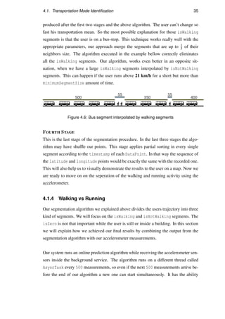
The algorithm can be further optimized by eliminating some relatively small segments
(but bigger than minimumSegmentSize) between really large segments. It is easier to
understand this with an example. Lets assume that Figure 4.6 shows the segmentList

45. 4.1. Transportation Mode Identification 35
produced after the first two stages and the above algorithm. The user can’t change so
fast his transportation mean. So the most possible explanation for those isWalking
segments is that the user is on a bus-stop. This technique works really well with the
appropriate parameters, our approach merge the segments that are up to 1
5 of their
neighbors size. The algorithm executed in the example bellow correctly eliminates
all the isWalking segments. Our algorithm, works even better in an opposite sit-
uation, when we have a large isWalking segments interpolated by isNotWalking
segments. This can happen if the user runs above 21 km/h for a short but more than
minimumSegmentSize amount of time.
Figure 4.6: Bus segment interpolated by walking segments
FOURTH STAGE
This is the last stage of the segmentation procedure. In the last three stages the algo-
rithm may have shuffle our points. This stage applies partial sorting in every single
segment according to the timestamp of each DataPoint. In that way the sequence of
the latitude and longitude points would be exactly the same with the recorded one.
This will also help us to visually demonstrate the results to the user on a map. Now we
are ready to move on on the seperation of the walking and running activity using the
accelerometer.
4.1.4 Walking vs Running
Our segmentation algorithm we explained above divides the users trajectory into three
kind of segments. We will focus on the isWalking and isNotWalking segments. The
isZero is not that important while the user is still or inside a building. In this section
we will explain how we achieved our final results by combining the output from the
segmentation algorithm with our accelerometer measurements.
Our system runs an online prediction algorithm while receiving the accelerometer sen-
sors inside the background service. The algorithm runs on a different thread called
AsyncTask every 500 measurements, so even if the next 500 measurements arrive be-
fore the end of our algorithm a new one can start simultaneously. It has the ability

46. 36 Chapter 4. Implementation and Development
to count the number of the norm values of x, y and z that are above a custom bound.
The bound was produced by analyzing more than 50 different accelerometer measure-
ments of walking and running. Figure 4.7 demonstrates two samples of walking and
running, holding the phone in every kind of different angle and pocket for objective
results. It is clear from the graph, and the two black horizontal lines we draw, that
when the majority of the norm values are more than 24 the users activity it has to be
running. In addition, we observed than the best results comes up when the number of
norm values larger our bound is more than 1
10 of the whole values. In particular, in
our implementation the 1
10 of the 500 values is 50. After the execution of our algo-
rithm we store the mean value of all norms, start and end time of the measurement
along with the result of the detection (notRunning or running). We add them in an
Collections.synchronizedList while our threads may run concurrently and at the
end we store them in our database.
Figure 4.7: Accelerometer measurements for walking and running
4.1.5 Identification
Now we are ready to produce our final results combining both the accelerometer and
segmentation techniques. Lets start with the isWalking segments from our final seg-
ment list. For every DataPoint there we extract the timestamp and then we check
whether or not it belongs in a running or notRunning sequence from our accelerom-
eter data. In particular, we traverse all the accelerometer records until we find one
that the given timestamp is between the start and end label. Then we can easily
determine the specific activity of this isWalking point. Figure 4.9 demonstrates the

47. 4.1. Transportation Mode Identification 37
implementation of the isThePointRunning() function. For better comprehension we
can see the function’s functionality as a filter for the dataPoints in figure 4.8.
Figure 4.8: Filtering the segmentation list using accelerometer measurements
The other isNotWalking segments from our segment list, means that the user is on
a vehicle. For rare circumstances that the user is a really good athlete that can run
more than 22km/h for a long distance may confuse our algorithm. However, the so-
lution to this problem is quite simple, we can use again the isThePointRunning()
function but now on the isNotWalking segments. If the result is running then the
user is running and if is notRunning then the user is on vehicle. Finally, for further
optimization when we observe an average speed more than 45 km/h we can be 100%
sure that the user is on vehicle. While 45 km/h is the fastest speed a human can achieve
(Usain Bolt, 100m sprint)1.
p r i v a t e boolean isThePointRunning ( long timeStamp ) {
f o r ( AccelerometerRunning aPoint : a c c e l e r o m e t e r L i s t ) {
i f ( timeStamp = aPoint . s t a r t timeStamp = aPoint . end )
i f ( aPoint . running == 1)
r e t u r n t r u e ;
e l s e
r e t u r n f a l s e ;
}
r e t u r n f a l s e ;
}
Figure 4.9: Function for filtering running and notRunning points
In the next section we will discuss an alternative machine learning technique to identify
our segments using classification.
1http://www.livescience.com/8039-humans-run-40-mph-theory.html

48. 38 Chapter 4. Implementation and Development
4.1.6 Classification
Classification is a machine learning technique that on the basis of a training set of
data containing observations, has the ability to identify to which of the existing set of
categories the new observation belongs. In our implementation we use already exist-
ing GPS recorded trajectories as a training set, and then we will try to determine the
transportation mode using different classifiers and algorithms. We achieved an overall
accuracy of around 83%.
To achieve this we used WEKA as our primary machine learning software. WEKA supports
multiple data mining techniques like data clustering, classification, regression and vi-
sualization. All those techniques are predicated on the assumption that the dataset is
available as one file (.ARFF) where each datapoint is described by a fixed number of
attributes. Bellow we can see our strategy in three signle steps.
1. Creating the data set file for training
2. Creating and exporting a new model
3. Reload this model to run against new data sets
4.1.7 Dataset Creation
For our training dataset we will use the speed measurements as we did in our seg-
mentation algorithms. We used Geolife GPS data in combination with our custom
collected data. Geolife is an already existing GPS trajectory dataset with latitude and
longitude coordinates along with a timestamp that was collected in by 182 users in a
period of over three years (from April 2007 to August 2012). This dataset contains
17,621 trajectories with a total distance of 1,292,951km and a total duration of 50,176
hours. However, only the 30% of those data containing information about the trans-
portation mode. There is an extra file called labels.txt with the following format
that contains useful information about the transportation mode for each trajectory.
2008/03/30 08:20:50 2008/03/30 08:37:01 car
2008/03/30 08:45:43 2008/03/30 10:09:13 car
2008/03/30 10:38:13 2008/03/30 11:02:45 walk
In order to properly parse those values we created a java application using Eclipse that

49. 4.1. Transportation Mode Identification 39
has the ability to aggregate the data according to their labels. So we started parsing
some of the trajectories with the label walk and simultaneously extracting the speed
from those points in the same way we explained in section 4.1.2. Subsequently, we
parsed the data with labels car, bus or taxi assuming that all belong in the same
category driving. In addition, we added the data collected from the extra android
application we created for manually storing the correct data for testing. The result was
to have a large file with speed values followed by the category walking or driving.
The next step was to create an .ARFF file with our dataset to access it through the
WEKA software. The generated file format can be seen below and it contains two at-
tributes. The speed in the specific point and a class attribute (walking or driving).
@relation activity recognition
@attribute speed numeric
@attribute class walking, driving
@data
4.300974848389722,walking
4.552357930824708,walking
5.317938399845843,driving
Now we can start using the WEKA software with the produced trained dataset file.
4.1.8 Create and Exporting Models
WEKA has the ability to generate and save models from the loaded dataset. It has also
the ability automatically test those models, using cross-validation. Cross-Validation
will not only use the whole data for training but a part of it like the 70% and the rest
30% would be for testing. In this way we can improve our accuracy without manu-
ally checking the results. We used multiple different classifiers like, Decision Trees,
Bayesian Network Model and Support Vector Machine to create our models. Each
model come from different algorithm approaches and will perform differently under
different data sets. After multiple tests we concluded that the most accurate model was
the Decision Trees with an accuracy of almost 83%.

50. 40 Chapter 4. Implementation and Development
4.1.9 Using The Model
Lets assume we have a new trajectory from our GPS with speed values and we want
to determine the category of each point using the generated model. We create a new
dataset with the following format:
@relation activity recognition
@attribute speed numeric
@attribute class walking, driving
@data
50.54,?
40,?
30,?
The classification algorithms will automatically replace all the question marks with
either driving or walking class. After we extracted our model in the .model file
we are ready to use it on new data sets. We can use both the WEKA API or the WEKA
Software. For instance, in WEKA Software we simply load our new data set and we re-
evaluate our model with the current data set. This option will automatically categorize
every single datapoint to the given classes. The following code will produce the same
results using the WEKA API so we can apply this machine learning technique inside on
our Android application:
C l a s s i f i e r c l a s s i f i e r = S e r i a l i z a t i o n H e l p e r . read ( ” dTrees . model ” ) ;
E v a l u a t i o n newTest = new E v a l u a t i o n ( d a t a S e t ) ;
newTest . evaluateModel ( c l a s s i f i e r , d a t a S e t ) ;
4.2 Processes and Communication
In this section we will discuss the communication between our threads, services and
the database. We will focus on the implementation of our foreground service. We
will also discuss the way we applied our transportation mode detection algorithms and
demonstrate the results in the view recording activity.

51. 4.2. Processes and Communication 41
4.2.1 Foreground Service
Foreground Service is responsible for the main business logic of the application. The
service has the following functionalities:
Receiving data from the GPS
Receiving data from the Accelerometer Sensor
Interacting with Google APIs
Running online expensive algorithms
Reading/Writing to the database
Interactive communication with external Activities
Create and editing the notification bar
The challenge was to combine all those features together to work smoothly and effi-
ciently with each other. We created a function called isServiceRunning() that has
the ability to examine if our foreground service is already running or not. In that way
even when the user closes the application completely it can continue/open the existing
service instead of creating a new service twice.
At the beginning of our service we initialize every component and data structure we
will need and we create the notification bar. In addition, a request to the user to enable
the GPS is popped up using the AlertDialog2 class. We use the onStartCommand()3
function because it provide us with the ability to interact with the service in real time
using Intents4 and Flags from other Activities or APIs. This function can distinguish
the different types of requests (actions from an Intent) that receives and respond with
the desired functionality. For instance, it can differentiate the service creation, start,
pause, request and update the current trajectory, receiving Google Activity recognition
results and communicate with the notification bar.
Furthermore, the service can simultaneously receive data and measurements from the
GPS and Accelerometer and store them in the database using threads and thread safe
2https://developer.android.com/reference/android/app/AlertDialog.html
3https://developer.android.com/reference/android/app/Service.html#onStartCommand
4https://developer.android.com/reference/android/content/Intent.html

52. 42 Chapter 4. Implementation and Development
data types like Collections.synchronizedList. It can communicate with other
activities and send the requested data via broadcasts5. Broadcasts is an efficient asyn-
chronous way of communication between activities while they can sent/receive almost
all kind of data types and can be used even from threads. Furthermore, our application
checks if the required permissions are granted before applying any action, so the user
would know exactly what device resources our application is using.
It was really challenging to create a service that could run in the background indef-
initely and at the same time the user to have the complete control of it. The ser-
vice can only have one instance and can not be closed even if the user swipe to
close the application from the devices menu. In that way the background service will
continue working and providing the notification bar when application is closed. To
achieve this we used the START STICKY6 option (that enables the system to re-create
our service after it is killed) on the creation of the service in combination with the
android:stopWithTask=false option in the android manifest. Finally, we have im-
plemented the appropriate distructors so when the user closes the service, everything
would be closed and stored to the database smoothly. To achieve this we override two
functions the onDestroy() and onTaskRemoved().
4.2.2 View Recording
At first the activity, receives the selected RECORDING ID from the list with all the
recordings. This is done by adding the appropriate information in a Bundle7 that can
parse different kind of objects in a new activity.
The first step is to obtain the whole GPS and Accelerometer data from our database
as well as the data from the Google Activity Recognition API. For performance op-
timization we implemented an AsyncTask thread in order to protect the GUI from
freezing. The following functions in Figure 4.10 are called from the Asynctask
doInBackground() function and run the appropriate queries to our database. They
reply with a Cursor8 object that contains the selected columns and rows.
5https://developer.android.com/reference/android/content/BroadcastReceiver.html
6https://developer.android.com/reference/android/app/Service.html
7https://developer.android.com/reference/android/os/Bundle.html
8https://developer.android.com/reference/android/database/Cursor.html

53. 4.3. Reducing Battery Consumption 43
Cursor c1 , c2 , c3 ;
db . open ( ) ;
c1 = db . getAccelerometerData (RECORDING ID) ;
c2 = db . getGpsData (RECORDING ID) ;
c3 = db . getGoogleData (RECORDING ID) ;
db . c l o s e ( ) ;
Figure 4.10: Retrieving the stored data from database
The second step is to execute our transpiration mode identification algorithms like seg-
mentation and classification, from within the same AsyncTask doInBackground()
function. After the completion of the recognition we parse the final results in the
onPostExecute() function that is responsible to communicate with the UI Thread
and visually demonstrate the results to the user. The results are demonstrated in a map
by combining and merging multiple polylines and circles with regard to the zIndex
that is the depth of our shapes. In addition, we store all those shapes in vectors so
that we can easily modify our map with the users choices. We created the whole map
representation ourselves without using any external library that might cause problems.
(we developed over 400 lines of code for the interactive map visualization)
4.3 Reducing Battery Consumption
The main problem in every recent application that uses high demanding operations
and multiple device features like Camera, GPS and Sensors is that consumes too much
battery. We don’t want this to our application while the users will avoid using it. We
use the following techniques to temper the battery consumption.
1. We store things on demand in our database (for example every N measurements)
in that way we avoid to access the database every second that can be energy
consuming.
2. We used the latest android available features to obtain Location data from GPS,
4G and Wi-Fi, where the user can even choose between accuracy or battery con-
sumption. For instance, if the user choose High Accuracy the system would
combine all those three features to provide the most accurate results. Contrary,
if the user selects Battery Saving mode we would try to determine the location
without using the GPS at all but there would be a dramatically drop in accuracy.

54. 44 Chapter 4. Implementation and Development
3. We tried not to overload our background service workload with needless calcu-
lations. For instance, we avoid calculating statistics in real time. Furthermore,
the application would consume less battery when the application is closed and
the foreground service is ruining by itself while the service would not have to
update live the application.
4. We inserted some delay on the GPS data receiving frequency. For example in-
stead of updating every 1 second we can receive data every 2 seconds or even
more. Exactly the same technique applied on the accelerometer, we tried to
reduce the amount of sensors generated data per second with respect to the ac-
curacy.
4.4 User Interface
In this section we demonstrate the interface design techniques and patterns we used to
make our user interface attractive to the users. The GUI evaluation is quite subjective
and requires a lot of test users. We tried to create a clear, responsive, attractive and
efficient application. The basic idea is that if our system is pleasant to use, users will
not simply be using it but instead they will look forward to using it.
CLARITY
Clarity is one of the most important elements for a successful UI design. We tried to
be clear in our buttons and elements by containing the whole information of the but-
tons tersely. In addition, every button has a description on long press that explains its
functionality (Figure 4.11. We avoid using fancy names and buttons so the user would
be able to know exactly what is the desired functionality. We used multiple colors and
lines on our map representation to be easy and clear for the user to differentiate the
different kind of transportation activities.
Figure 4.11: Description on long press click for clarity

55. 4.4. User Interface 45
RESPONSIVENESS
Responsive means that the application should work fast. Freezing screens, slow load-
ing times and interfaces leads to user dissatisfaction. A responsive interface that load
quickly improves the user experience. To achieve this we used multiple Threads,
AsyncTasks and Services on every long-running operation we used (read/write database,
segmentation, simplification and classification) to reduce the workload on the UI Thread.
In android development having a lightweight UI Thread improves the response dra-
matically. We also achieved high responsiveness by showing the appropriate messages
to the user. For instance, if the GPS is disabled we help him to enable it.
EFFICIENCY
An efficient UI should perform the appropriate functions and methods as fast as pos-
sible. The selection of the algorithms and the execution sequence is really important
to achieve efficiency. In our implementation we used multiple techniques to achieve
this. Our database doesn’t have needless data and redundancies in order to execute
queries faster. An example is that we store the mean value every 500 accelerometer
measurements instead of every single one of them. Another technique we applied is
the use of BroadcastReceivers we discussed in section 4.2 for efficient communica-
tion between activities. We also used the new Google feature RecyclerView9 instead
of ListView. The RecyclerView is much more powerful, flexible and a major en-
hancement over ListView. The main benefit is the caching that can result a smooth
scrolling experience to the users. Finally, we used our custom notification bar to pro-
vide the user with the ability to interact with the application even if he is out of the
applications scope.
ATTRACTIVENESS
Attractiveness is the last but really important feature we used to improve our UI. We
imported custom libraries to add animations in multiple parts of the application in or-
der to be interactive and satisfying to use. We also used custom libraries to improve the
appearance of the buttons while we used the latest Android features like Toolbars10,
9https://developer.android.com/reference/android/support/v7/widget/RecyclerView.html
10https://developer.android.com/reference/android/widget/Toolbar.html

56. 46 Chapter 4. Implementation and Development
CardViews11 for proficient result. We also used smooth colors that would be famil-
iar with the user. Figure 4.12 demonstrate the different colors we used to infer each
activity. Finally, we used custom readable fonts and a starting splash screen.
Figure 4.12: Correlation between colors and transportation modes
11https://developer.android.com/reference/android/support/v7/widget/CardView.html

57. Chapter 5
Evaluation
In this chapter we evaluate the accuracy of our transportation mode identification al-
gorithms using manually collected data as well as the Geolife dataset. At fist, We
explain how we chose our parameters for our techniques. Next we will demonstrate
the accuracy of our segmentation technique. We observed an impressive overall accu-
racy of 85% while for differentiating walking with running 95%! Subsequently, we will
evaluate our classification algorithms that achieved an accuracy of about 83%. We also
compare those results with the activity recognition from Google API. Finally, we will
examine the battery consumption of the application.
5.1 Parameter Selection
To find the appropriate and most efficient values for our parameters we used the fol-
lowing strategy. For segmentation, lets assume we want to find the best values for
minimumSegmentSize and speedUpperBound. We created a simple program that exe-
cutes the Segmentation algorithm with different values each time and then we compare
the results. We used the values that produced the most accurate results. For instance,
minimumSegmentSize = 30 produced the highest accuracy of about 95% for iden-
tifying isWalking and isNotWalking segments while minimumSegmentSize = 20
produced an accuracy of 80%.
The accelerometer boundaries selection was more challenging. We used the Python
programming language with matplotlib to create plots using the norm measurements
we demonstrated in section 4.1.4 from the accelerometer and conclude to the most ef-
ficient values after multiple tests with more than 20 hours of data. We also compared
those values with a different mobile device for objectivity purposes.
47

58. 48 Chapter 5. Evaluation
5.2 Accuracy and Tests Using Segmentation
5.2.1 Real Life
We have done more than 120 different tests to observe our results and accuracy. The
main tests where made using the smartphone Google Nexus 5X with version Marshmallow
6.0.1 while complementary tests have been done using the Samsung Galaxy S5 with
version Lollipop 5.0.2. We used the second mobile device to examine that every-
thing works fine no matter the hardware and the operating system we got. To investi-
gate and compare our accuracy we created another simple application, that could help
us manually store the actual-real activity along with a timestamp.
Walking vs Running
The identification of those two activities was mainly done by the accelerometer. The
accuracy we achieved is quite impressive and around 95%. We did more than 50 dif-
ferent tests for walking and running. In those tests we had the phone inside a pocket,
inside a bag or we were holding it. Figure 5.1 illustrate three really long complected
routes of an overall distance of 11 km that we walked at the same day with an ac-
curacy of 99.9%! The error was only 100 meters. While Figure 5.2 demonstrates
our long jogging travel of around 2km with an accuracy of 99%. We can clearly see
that walking and running identification works perfect. However, we observed that in
abruptly downhills and stairs when the users have the phone in his pocket and walks
quite fast may confuse our algorithm, that is why our accuracy fell to 95%.
Figure 5.1: 11 km of pure walking achieved 99.9% accuracy

59. 5.2. Accuracy and Tests Using Segmentation 49
Figure 5.2: 2 km of pure running achieved 99% accuracy
Walking vs Running vs Vehicle
The accuracy we observed identifying all the three transportation modes simultane-
ously was about 85%. However, the main vehicle we used for testing our algorithms
was the bus. We chose the bus because if our identification works there then we can be
sure that it will also work with all the other vehicles like cars, trains and motorcycles.
This is because our algorithms mostly depend on speed measurements and buses have
multiple stops so they can’t move that fast, the fastest the vehicle travels the easiest the
identification. We did more than 20 tests using bus and around five tests using cars.
The most common recorded accuracy is around 90%. However, traffic and especially
traffic jams affect the accuracy and can be from 75% to 85%. The problem is that it is
almost impossible to differentiate if a vehicle is moving really slow or the users walks
with high accuracy. To overwhelm, this problem we might have to use more sensors.
Figure 5.3a demonstrates the original route where the blue polyline means that the
user is walking and the green that is in a vehicle (in our example a bus). Figure 5.3b
shows our identification results. First of all, we can observe that the original walking
segments at the start are 100% correct. Now we can see the problem is in the middle
of our bus trip between the two black parallel lines we draw, while there was a lot of
traffic there. So the whole trip was about 11km and the error segment was about 2km,
so we can see that 9
11km where correct. As a result our accuracy is about 81%.

60. 50 Chapter 5. Evaluation
(a) Original Route Activities (b) Identification Results
Figure 5.3: 10km on a bus with some traffic achieved 81% accuracy
5.2.2 Simulation
We used our parsing program we described in section 4.1.7 to load and transform
the Geolife dataset. However, instead of creating the .arff files we executed our
segmentation algorithms on those data. We transferred our segmentation algorithms
from Android Studio to Eclipse for further examination of the results. Our overall
data test consists of around 19170 lines of vehicle (10748) and walking (8422) GPS
measurements. We should note here that unfortunately Geolife dataset does not pro-
vide accelerometer measurements to improve our identification algorithms. Figure 5.4
demonstrates the results after the execution. We achieved an overall accuracy of around
84% as we expected from our real life tests in 5.2.1. In particular, 16168
19170 = 0.84 of the
data points were identified correctly.

61. 5.3. Classification 51
Figure 5.4: Segmentation results from Geolife trajectory (19170 points)
5.3 Classification
Classification is the mainly used technique for the transportation mode identification
using a trained data set. We will use the .ARFFF file we created in section 4.1.7 as
our training data set. The produced file contains exactly the same data we used in our
simulation above but in a different format in order to be recognized from the WEKA
software. We used multiple classifiers to achieve the most accurate results. The clas-
sifiers that produced the most efficient results were the Decision Trees, Bayesian
Network and the Support Vector Machine. Table 5.1 demonstrates the accuracy of
those methods using 10 fold cross-validation on our 19170 number of data points. We
can clearly see that most efficient method is using Decision Trees with 83% accu-
racy.
Method Correctly Classified Instances Accuracy
Decision Trees 15336 83%
Support Vector Machine 15144 79%
Bayesian Network 14377 75%
Locally weighted learning 14185 74%
Naive Bayes 13610 71%
Simple Logistic 13419 70%
Table 5.1: Classification results using 10 fold cross-validation and different classifiers

62. 52 Chapter 5. Evaluation
In addition, We exported the most accurate Decision Trees model and we made
further tests by re-evaluating our model with new smaller data-sets. The accuracy we
observed was around 78% to 83% as we expected from our cross-validation tests.
5.4 Comparison with Google API
The first step was to retrieve our stored data from the database about the Activity
Recognition from the API. For every record, we retrieved the timestamp along with
the activity and we placed the results in a sorted list according timestamp. Now, for
every point in our trajectory we try to find the closest and minimum value inside the
list we just created. In that way we could obtain the activity that Google API identified
that specific time. Figure 5.5 demonstrates the sample code we used to achieve this.
p r i v a t e boolean isThePointGoogleVehicle ( long timeStamp ) {
GoogleData prev = n u l l ;
f o r ( GoogleData a c cP o in t : googleDataList ) {
i f ( timeStamp a cc P oi n t . timestamp prev != n u l l ) {
Log . i (TAG, prev . a c t i v i t y ) ;
i f ( prev . a c t i v i t y . equals ( ” In Vehicle ” ) )
r e t u r n t r u e ;
e l s e
r e t u r n f a l s e ;
}
prev = a cc P oi n t ;
}
r e t u r n f a l s e ;
}
Figure 5.5: Function for filtering in vehicle points according to Google API
Activity Recognition using Google API has a lot of problems. We observed that it
can not recognize the human activity running but instead recognize it as On Foot or
Tilting. So our implementation has an advantage to infer walking and running.
This was expected while the Google API doesn’t use the accelerometer.
We also observed that after 10 recorded trips with a bus it recognized that the user
is on vehicle with only about 65% accuracy. While our segmentation algorithm had an
accuracy of almost 80%. The next Figure 5.6 shows an example of one of the trips

63. 5.5. Battery Consumption 53
were the black dots represent the Google API In vehicle recognition. The difference
is extraordinary, our algorithm there achieved an accuracy of 97% while the Google
API had an overall 65% in recognizing the In Vehicle trajectory.
(a) Segmentation (b) Google API
Figure 5.6: Our approach versus Google API
5.5 Battery Consumption
Heavy demanding operations like segmentation in combination with GPS and Ac-
celerometer sensors consumes a lot of battery. This has a great impact on users of
the application because it would repel them from using it. We tested our application
to observe the battery consumption. Figure 5.7 demonstrate the results after 1 hour
of running. The results are impressive while after 1 hour of running the application
consumed only 2% of the whole battery.

64. 54 Chapter 5. Evaluation
(a) 2% consumption after one hour running (b) Hardware Consuption
Figure 5.7: Battery consumption

65. Chapter 6
Conclusion and Future Work
In this Thesis, we developed a framework that has the ability to identify different trans-
portation modes. The challenge was to achieve high accuracy results in an efficient
and user friendly way. Specifically, we analyzed and examined the already existing
approaches that are commonly used for this problem in order to improve our knowl-
edge and techniques. We started by designing our system’s architecture with respect to
efficiency, usability and scalability. Next, we implemented our architecture using the
latest android development techniques while we also exploited the power of several
third-party tools. Subsequently, we created the relational database of the system. After
that we implemented the main logic and algorithms for our transportation mode detec-
tion and we finished our application by using some techniques and patterns to achieve
an interactive and appealing user interface. The evaluation of the system and the com-
parison of it with popular ML classification techniques showed that our segmentation
technique produce more accurate results. The reason is because our segmentation im-
plementation is created for this specific kind of problem while the classification al-
gorithms we used are not implemented for this particular problem. We achieved an
overall accuracy of 85%. We also observed that our implementation works better than
the new Google API for activity recognition. We observed 0% crashes and the appli-
cation worked smoothly in multiple smartphones.
A problem we observed is that our accuracy decreases when there is a lot off traf-
fic. Another approach could possibly try to solve this problem by analyzing the GPS
and accelerometer measurements on traffic jams and improve the accuracy even more.
In addition, we could increase the classification attributes by adding more information
about the trips. Another interesting improvement that can be done is to add a score
55

66. 56 Chapter 6. Conclusion and Future Work
calculator on our application, that is efficiently increased every time the user uses the
application. So the more the use of the application the larger the users score. In that
way we will attract more people to use our application. Finally, it would be interest-
ing to transform the whole functionality of our Android application framework to a
wearable device like a smart watch. This will open up new prospects for accuracy
improvements while the position of the device would be fixed.

67. Bibliography
[1] Geoffrey Blewitt. Basics of the gps technique: observation equations. Geodetic
applications of GPS, pages 10–54, 1997.
[2] A Rajalakshmi and G Kapilya. The enhancement of wireless fidelity (wi-fi) tech-
nology, its security and protection issues. 2014.
[3] Ian Anderson and Henk Muller. Practical activity recognition using gsm data.
2006.
[4] Jonny Farringdon, Andrew J Moore, Nancy Tilbury, James Church, and Pieter D
Biemond. Wearable sensor badge and sensor jacket for context awareness. In
Wearable Computers, 1999. Digest of Papers. The Third International Sympo-
sium on, pages 107–113. IEEE, 1999.
[5] Cliff Randell and Henk Muller. Context awareness by analysing accelerometer
data. In Wearable Computers, The Fourth International Symposium on, pages
175–176. IEEE, 2000.
[6] Ling Bao and Stephen S Intille. Activity recognition from user-annotated accel-
eration data. In International Conference on Pervasive Computing, pages 1–17.
Springer, 2004.
[7] Raghu K Ganti, Praveen Jayachandran, Tarek F Abdelzaher, and John A
Stankovic. Satire: a software architecture for smart attire. In Proceedings of
the 4th international conference on Mobile systems, applications and services,
pages 110–123. ACM, 2006.
[8] Nicky Kern, Bernt Schiele, and Albrecht Schmidt. Multi-sensor activity context
detection for wearable computing. In European Symposium on Ambient Intelli-
gence, pages 220–232. Springer, 2003.
57

68. 58 Bibliography
[9] T Saponas, Jonathan Lester, Jon Froehlich, James Fogarty, and James Landay.
ilearn on the iphone: Real-time human activity classification on commodity mo-
bile phones. University of Washington CSE Tech Report UW-CSE-08-04-02,
2008, 2008.
[10] Juha Parkka, Miikka Ermes, Panu Korpipaa, Jani Mantyjarvi, Johannes Peltola,
and Ilkka Korhonen. Activity classification using realistic data from wearable
sensors. IEEE Transactions on information technology in biomedicine, 10(1):
119–128, 2006.
[11] Miikka Ermes, Juha P¨arkk¨a, Jani M¨antyj¨arvi, and Ilkka Korhonen. Detection of
daily activities and sports with wearable sensors in controlled and uncontrolled
conditions. IEEE Transactions on Information Technology in Biomedicine, 12
(1):20–26, 2008.
[12] Sunny Consolvo, David W McDonald, Tammy Toscos, Mike Y Chen, Jon
Froehlich, Beverly Harrison, Predrag Klasnja, Anthony LaMarca, Louis
LeGrand, Ryan Libby, et al. Activity sensing in the wild: a field trial of ubifit gar-
den. In Proceedings of the SIGCHI Conference on Human Factors in Computing
Systems, pages 1797–1806. ACM, 2008.
[13] Jonathan Lester, Tanzeem Choudhury, and Gaetano Borriello. A practical ap-
proach to recognizing physical activities. In International Conference on Perva-
sive Computing, pages 1–16. Springer, 2006.
[14] David P Wagner. Lexington area travel data collection test: Gps for personal
travel surveys. Final Report, Office of Highway Policy Information and Office
of Technology Applications, Federal Highway Administration, Battelle Transport
Division, Columbus, 1997.
[15] Geert Draijer, Nelly Kalfs, and Jan Perdok. Global positioning system as data
collection method for travel research. Transportation Research Record: Journal
of the Transportation Research Board, (1719):147–153, 2000.
[16] Jean Wolf, Randall Guensler, and William Bachman. Elimination of the travel
diary: Experiment to derive trip purpose from global positioning system travel
data. Transportation Research Record: Journal of the Transportation Research
Board, (1768):125–134, 2001.

69. Bibliography 59
[17] Timothy Forrest and David Pearson. Comparison of trip determination methods
in household travel surveys enhanced by a global positioning system. Transporta-
tion Research Record: Journal of the Transportation Research Board, (1917):
63–71, 2005.
[18] Joshua Auld, Chad Williams, Abolfazl Mohammadian, and Peter Nelson. An
automated gps-based prompted recall survey with learning algorithms. Trans-
portation Letters, 1(1):59–79, 2009.
[19] Zahra Ansari Lari and Amir Golroo. Automated transportation mode detection
using smart phone applications via machine learning: case study mega city of
tehran. In Transportation Research Board 94th Annual Meeting, number 15-
5826, 2015.
[20] Sasank Reddy, Min Mun, Jeff Burke, Deborah Estrin, Mark Hansen, and Mani
Srivastava. Using mobile phones to determine transportation modes. ACM Trans-
actions on Sensor Networks (TOSN), 6(2):13, 2010.
[21] Chao Xu, Minhe Ji, Wen Chen, and Zhihua Zhang. Identifying travel mode from
gps trajectories through fuzzy pattern recognition. In Fuzzy Systems and Knowl-
edge Discovery (FSKD), 2010 Seventh International Conference on, volume 2,
pages 889–893. IEEE, 2010.
[22] Timothy Sohn, Alex Varshavsky, Anthony LaMarca, Mike Y Chen, Tanzeem
Choudhury, Ian Smith, Sunny Consolvo, Jeffrey Hightower, William G Griswold,
and Eyal De Lara. Mobility detection using everyday gsm traces. In International
Conference on Ubiquitous Computing, pages 212–224. Springer, 2006.
[23] M Mun, Deborah Estrin, Jeff Burke, and Mark Hansen. Parsimonious mobility
classification using gsm and wifi traces. In Proceedings of the Fifth Workshop on
Embedded Networked Sensors (HotEmNets), 2008.
[24] John Krumm and Eric Horvitz. Locadio: Inferring motion and location from wi-fi
signal strengths. In Mobiquitous, pages 4–13, 2004.
[25] Kavitha Muthukrishnan, Maria Lijding, Nirvana Meratnia, and Paul Havinga.
Sensing motion using spectral and spatial analysis of wlan rssi. In European
Conference on Smart Sensing and Context, pages 62–76. Springer, 2007.

70. 60 Bibliography
[26] Adel Bolbol, Tao Cheng, Ioannis Tsapakis, and James Haworth. Inferring hybrid
transportation modes from sparse gps data using a moving window svm classifi-
cation. Computers, Environment and Urban Systems, 36(6):526–537, 2012.
[27] Leon Stenneth, Ouri Wolfson, Philip S Yu, and Bo Xu. Transportation mode de-
tection using mobile phones and gis information. In Proceedings of the 19th ACM
SIGSPATIAL International Conference on Advances in Geographic Information
Systems, pages 54–63. ACM, 2011.
[28] Lijuan Zhang, Sagi Dalyot, Daniel Eggert, and Monika Sester. Multi-stage ap-
proach to travel-mode segmentation and classification of gps traces. In Proceed-
ings of the ISPRS Guilin 2011 Workshop on International Archives of the Pho-
togrammetry, Remote Sensing and Spatial Information Sciences, Guilin, China,
volume 2021, page 8793, 2011.
[29] Yu Zheng, Like Liu, Longhao Wang, and Xing Xie. Learning transportation mode
from raw gps data for geographic applications on the web. In Proceedings of the
17th international conference on World Wide Web, pages 247–256. ACM, 2008.
[30] P Gonzalez, J Weinstein, S Barbeau, M Labrador, P Winters, Nevine Labib
Georggi, and Rafael Perez. Automating mode detection using neural networks
and assisted gps data collected using gps-enabled mobile phones. In 15th World
congress on intelligent transportation systems, 2008.
[31] Tao Feng and Harry JP Timmermans. Transportation mode recognition using gps
and accelerometer data. Transportation Research Part C: Emerging Technolo-
gies, 37:118–130, 2013.
[32] Vincenzo Manzoni, Diego Maniloff, Kristian Kloeckl, and Carlo Ratti. Trans-
portation mode identification and real-time co2 emission estimation using smart-
phones. SENSEable City Lab, Massachusetts Institute of Technology, nd, 2010.
[33] Emiliano Miluzzo, Nicholas D Lane, Krist´of Fodor, Ronald Peterson, Hong Lu,
Mirco Musolesi, Shane B Eisenman, Xiao Zheng, and Andrew T Campbell. Sens-
ing meets mobile social networks: the design, implementation and evaluation of
the cenceme application. In Proceedings of the 6th ACM conference on Embed-
ded network sensor systems, pages 337–350. ACM, 2008.

71. Bibliography 61
[34] Toshiki Iso and Kenichi Yamazaki. Gait analyzer based on a cell phone with a
single three-axis accelerometer. In Proceedings of the 8th conference on Human-
computer interaction with mobile devices and services, pages 141–144. ACM,
2006.
[35] Samuli Hemminki, Petteri Nurmi, and Sasu Tarkoma. Accelerometer-based
transportation mode detection on smartphones. In Proceedings of the 11th ACM
Conference on Embedded Networked Sensor Systems, page 13. ACM, 2013.
[36] Nishkam Ravi, Nikhil Dandekar, Preetham Mysore, and Michael L Littman. Ac-
tivity recognition from accelerometer data. In AAAI, volume 5, pages 1541–1546,
2005.