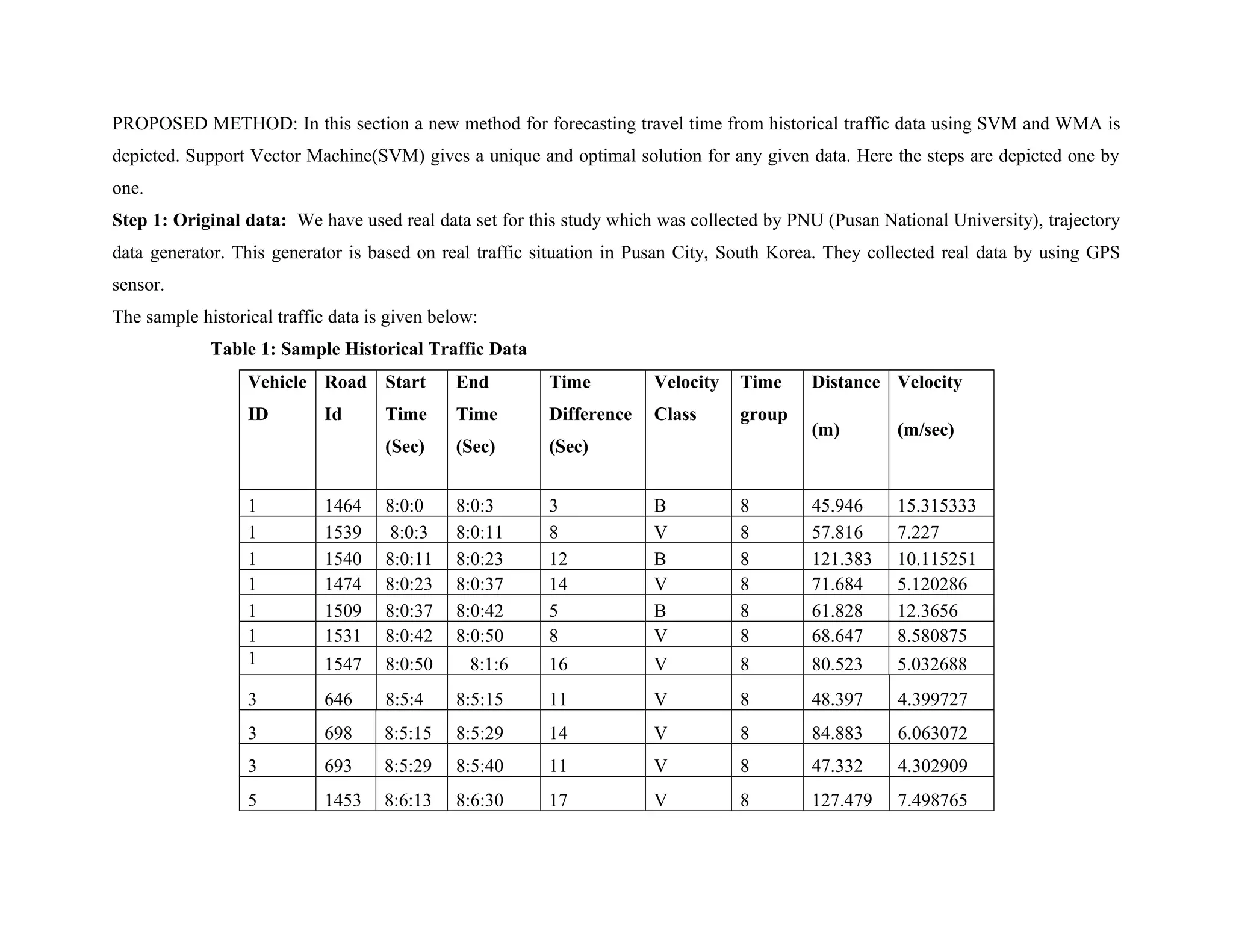
The document describes a new method for travel time prediction using support vector machine (SVM) and weighted moving average (WMA). It uses historical traffic data classified into velocity classes using SVM. It then predicts travel time using a modified WMA equation applied to the SVM support vectors. This method is compared to previous methods like successive moving average, chain average, and artificial neural network. Experimental results show the proposed SVM and WMA method performs better in terms of accuracy and computational complexity.

1. Travel Time Prediction using Support Vector Machine(SVM) and Weighted Moving Average(WMA)
ABSTRACT: Travel Time forecasting in highway system has appeared a vital issue for delivering travellers exact guidance about
choosing their route. In this paper, a new method for forecasting travel time from historical traffic data using SVM and WMA is
depicted. The proposed work has been divided into two parts: First one is classifying Travel Time depending on the traffic condition or
velocity class using Support Vector Machine(SVM) and Second one is predicting Travel Time using modified Weighted Moving
Average(WMA) method with a modified equation where the WMA method will be applied on the support vectors whose are
generated after classifying time using travel time Multi class all versus all SVM. Considering the same historical traffic data, the
outcomes of previous methods also compare with the outcome of propose method.In this case, previous methods include Successive
Moving Average (SMA), Chain Average (CA), and Artificial Neural Network (ANN). The comparison result proofs the better
performance of SVM and WMA method than the previous methods.
Keywords: Intelligent Transportation System (ITS); Support Vector Machine (SVM); Weighted Moving Average (WMA); Successive
Moving Average (SMA); Chain Average (CA); Artificial Neural Network (ANN); Travel Time Prediction.
INTRODUCTION: Travelling means movement from one geographical location to another geographical location by travellers. Since
all time the condition of the road is not the same because of traffic flow or other reasons, so it is very important for the travellers to
choose the correct path during travelling. If the travellers can know the available route and current condition about the road they can
easily reach their destination. Therefore, Prediction of Travel Time is an important issue in the area of Intelligent Transport
System(ITS). Intelligent Transport Systems(ITS) are highly developed applications, seek to provide novel services about various
modes of transport and traffic administration and facilitate travellers to be up to date, more harmonized, and best use of transport
networks. With the improvement of Advanced Travellers Information System (ATIS) travel time Prediction is more and more
important issue as it guide tourists delivering their desired route information[1].For tourist satisfaction, the consistent and exact
prediction of travel time on street network has emerged a crucial role in any types of vivacious means guidance
system[2].Furthermore, the significance of travel time forecasting is very useful to find out the shortest path in order to tour time. The

2. features that are responsible for varying travel time are vehicle speed, traffic and weather condition and also incidence in roads[3].
Moreover, Travel time is also dependent on traffic flow because of busy time and free time[4]. That is, Time reliant feature of traffic
flow is also significant. As a result, in this problem area research is very essential for delivering reliable travel time information to
meet user’s target [5,6,7,8,9].
Numerous algorithms and methods have been recommended in forecasting travel time including time series analysis along with
techniques of data mining. Data mining is a computational process used to discover unique, incredible and valuable data from large
dataset. To determine frequent occurrences[10] (e.g., common pathways selected by tourists) and to seek out inconsistencies [11] (e.g.,
irregularly hectic travel time) the contribution of common data mining techniques is very appreciable. In addition to, there are other
data mining techniques available for forecasting travel time. For example, classification techniques[4] can be used for training
historical traffic data and for calculating exact travel time for unknown data. Likewise, based on a class of similar data, travel time
can be predicted by using clustering techniques[12].This techniques used to cluster or bunch the same types of data into the same
class. Last few years, a numerous procedures and algorithms have been developed[13,14,15] for forecasting travel time. For example,
in KES 2008 a classification process, Naïve Baysian Classifier NBC[4] is recommended and KES 2009 introduced two other
algothims SMA and CA[16] for same task. Moving average was the conception of these algorithms and the outcomes of these
methods were more perfect. MKC[12] which was a clustering algorithm proposed in KES 2010.It recovers the limitation of
SMA,CA[16] and NBC[4].Inspite of these, it has been found that some limitation still remaining in this methods. In this paper, an
innovative method using SVM and WMA is applied to calculate travel time exactly and accurately and this method performs better
than the previous methods. Analyzing experimental results, this method reveals satisfactory result in terms of cost and computational
complexity. Furthermore, it eliminates unwanted fluctuations in the data set in comparing to conventional moving average method.
In this article at first some discussions about this area are demonstrated. Then our proposed method is discussed and examined and
after this a comparison is made by MARE analysis. Finally, we conclude a fruitful conclusion.

3. Background Study: Intelligent Transportation System is an important research area in predicting travel time. Many researches have
been done in this are for forcasting travel time so that tourists can easily choose their desire route. Since last few years, a number of
methods and algorithms have been established for calculating travel time exactly and accurately and these approaches revealed
performance from different views. This section comprises related works about prediction of travel time. Artificial Neural Network
(ANN) suggested by Park et al [17,18] used to predict freeway corridor travel time. But it could not predict the link travel time. For
classification of traffic pattern contribution of Kohonen Self Organizing Feature Map (SOFM) and Fuzzy c-means is appreciable.
Considering gaps in traffic data Lint et al[19,20] proposed a state-space neural network based method for predicting travel time
exactly. Linear regression also performed better in travel time prediction which was proposed by Kwon et al[21]. Rice et
al[22]proposed a method to predict the time required to pass through a given time in upcoming day. Comparison between the results
(results of various travel time prediction methods) was made by Wu et al[23].In their paper they proposed Support vector regression
(SVR) and used real highway traffic data. A switching model consisting of two linear predictors also used in travel time prediction
proposed by Erick et al[24]. Considering the possible velocity level for any road segment, another method which was also scalable to
road networks with random travel routes named NBC was suggested by Lee et al[4].This paper also used historical traffic data.
Representing the knowledge as rules a Rule-based Bayesian classification(RBC) [25] also suggested. It was an extension of NBC.
Moving average was also another idea for travel time prediction and in this case Successive Moving Average (SMA) and Chain
Average (CA)[16]- were originated. MKC method was successfully applied by Nath et al.[12] for calculating travel time. It was a
clustering method where the data were grouped into a number of clusters and after this final travel time can be derived from the
average of the mean of travel times of each cluster. The contribution of MKC in travel time prediction was very appreciable for
addressing uncertain situations. Inspite of these, existing systems still contain some significant problems. For example weighted
moving average method use weight while moving average method does not use any weighted. The weighted moving average model
weight recent historical data more heavily than older data when determining the average. In this paper, our contribution was to recover
the limitations of earlier methods using our proposed SVM and WMA method.

4. PROPOSED METHOD: In this section a new method for forecasting travel time from historical traffic data using SVM and WMA is
depicted. Support Vector Machine(SVM) gives a unique and optimal solution for any given data. Here the steps are depicted one by
one.
Step 1: Original data: We have used real data set for this study which was collected by PNU (Pusan National University), trajectory
data generator. This generator is based on real traffic situation in Pusan City, South Korea. They collected real data by using GPS
sensor.
The sample historical traffic data is given below:
Table 1: Sample Historical Traffic Data
Vehicle
ID
Road
Id
Start
Time
(Sec)
End
Time
(Sec)
Time
Difference
(Sec)
Velocity
Class
Time
group
Distance
(m)
Velocity
(m/sec)
1 1464 8:0:0 8:0:3 3 B 8 45.946 15.315333
1 1539 8:0:3 8:0:11 8 V 8 57.816 7.227
1 1540 8:0:11 8:0:23 12 B 8 121.383 10.115251
1 1474 8:0:23 8:0:37 14 V 8 71.684 5.120286
1 1509 8:0:37 8:0:42 5 B 8 61.828 12.3656
1 1531 8:0:42 8:0:50 8 V 8 68.647 8.580875
1 1547 8:0:50 8:1:6 16 V 8 80.523 5.032688
3 646 8:5:4 8:5:15 11 V 8 48.397 4.399727
3 698 8:5:15 8:5:29 14 V 8 84.883 6.063072
3 693 8:5:29 8:5:40 11 V 8 47.332 4.302909
5 1453 8:6:13 8:6:30 17 V 8 127.479 7.498765

5. 5 1458 8:6:30 8:6:38 8 V 8 75.012 9.3765
5 1422 8:6:38 8:6:50 12 V 8 64.999 5.416584
5 1360 8:6:50 8:6:58 8 V 8 69.238 8.65475
In Table 1 there are nine columns. Each column indicates different feature of traffic data. Here a row has the remaining attributes like
Vehicle ID, Road ID, and Start time, End Time, Time Group, Distance, Velocity, and Velocity Class. Vehicle Id indicates a specific Id
for a vehicle. Road Id indicates vehicle starts from which Road and every road has a specific id. Two attributes Start Time and End
Time indicate period during when a vehicle travels on a particular road segment.
Velocity Class: Different velocity classes arise for vehicles at different time periods of a day. In a road network, the moving pattern of
vehicles is varied according to the change of time in a day. Due to this, from historical traffic data we can found that they divided road
segment velocity into three different. Let Velocity Class = {VB, B, F} be the set of velocity classes. The VB, B and F mean very busy,
busy and free, respectively. The velocity classes are shown in Table 1.
Time Difference: Time difference indicates difference between Start Time and End time which is also time in second.
Distance: Distance indicates distance between road segments.
Velocity: Velocity indicates velocity or speed of vehicles on which Velocity Class also depends.
From this historical traffic data with nine different attributes or features I have used only two attributes or features for predicting travel
time. These two attributes are Time Difference between start time and end time of a vehicle and another attribute is Velocity class.
Because I have used Time Differences with Velocity Class for foretelling travel time and then imported data to Matlab.
Table 2: Time and Velocity Class used as original Data

6. No Time
1 3
2 8
3 12
4 14
5 5
6 8
7 16
8 10
9 7
10 2
No Class
1 B
2 V
3 B
4 V
5 B
6 V
7 V
8 V
9 B
10 F

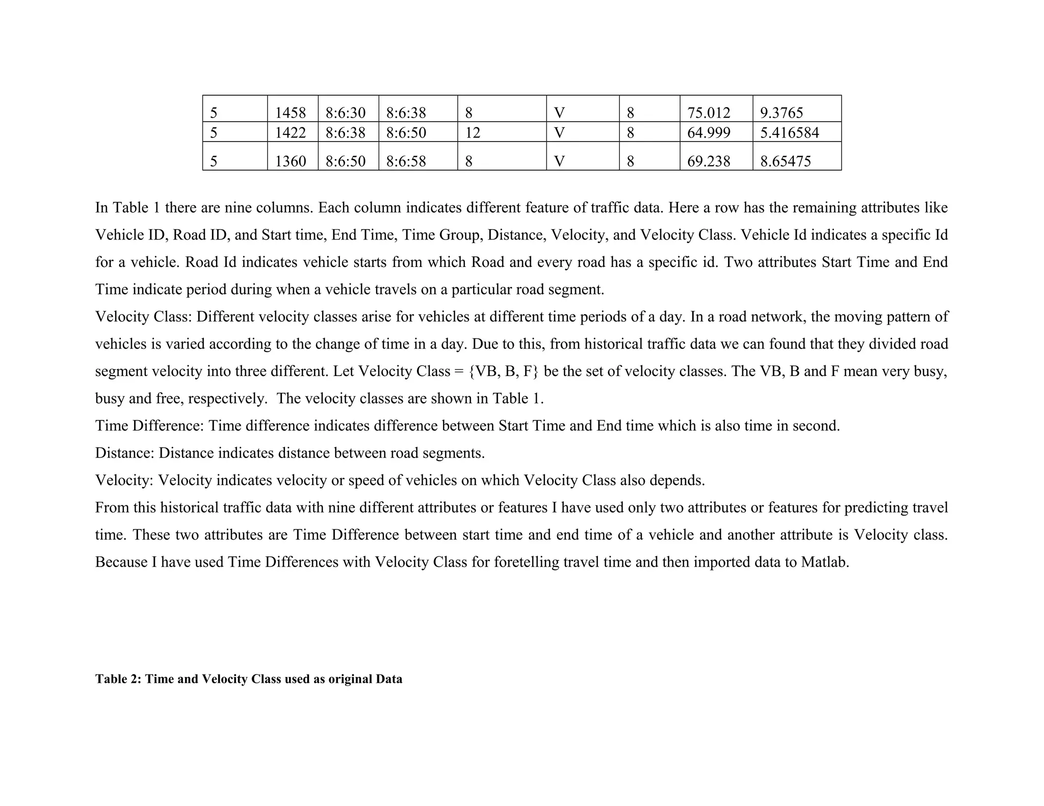
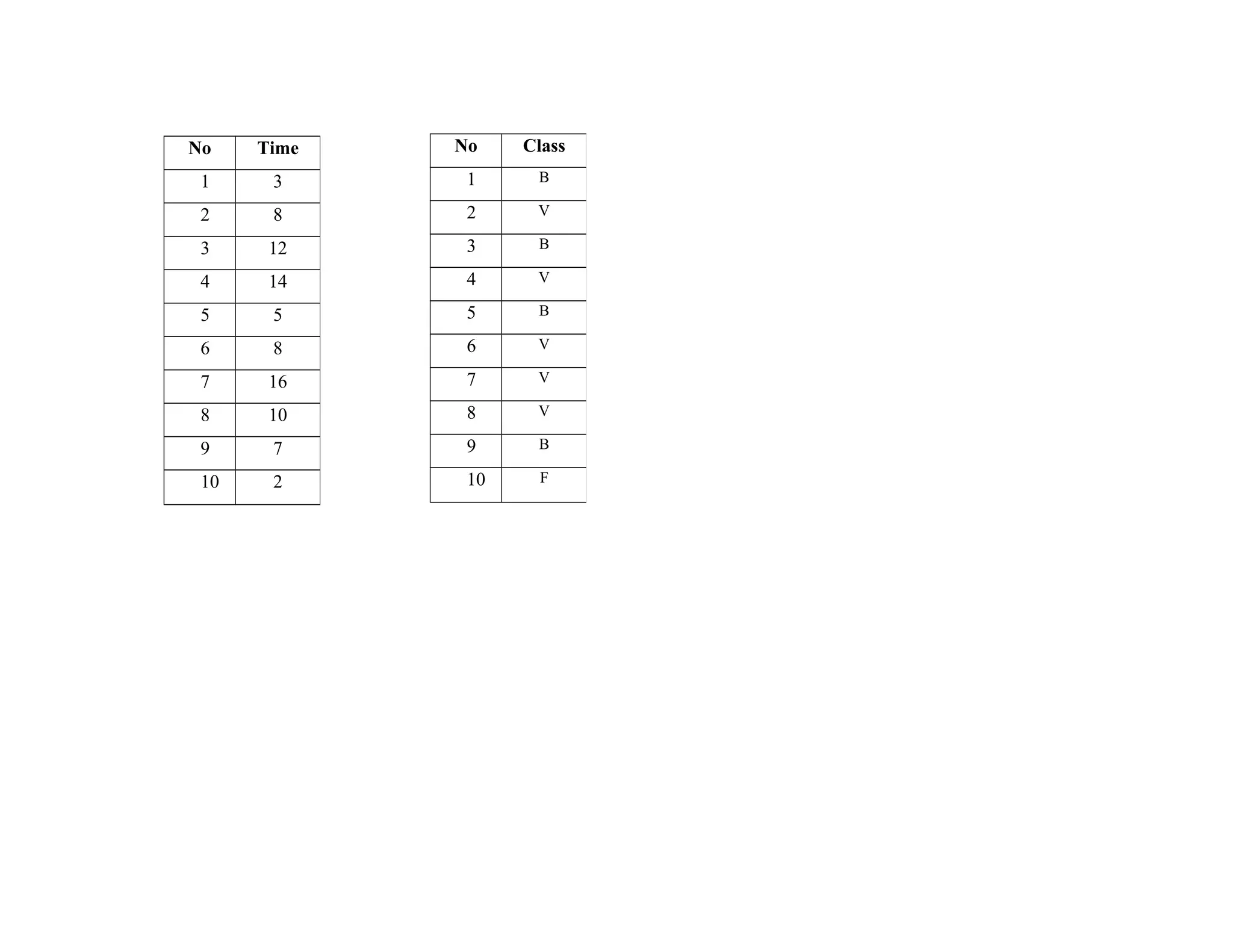
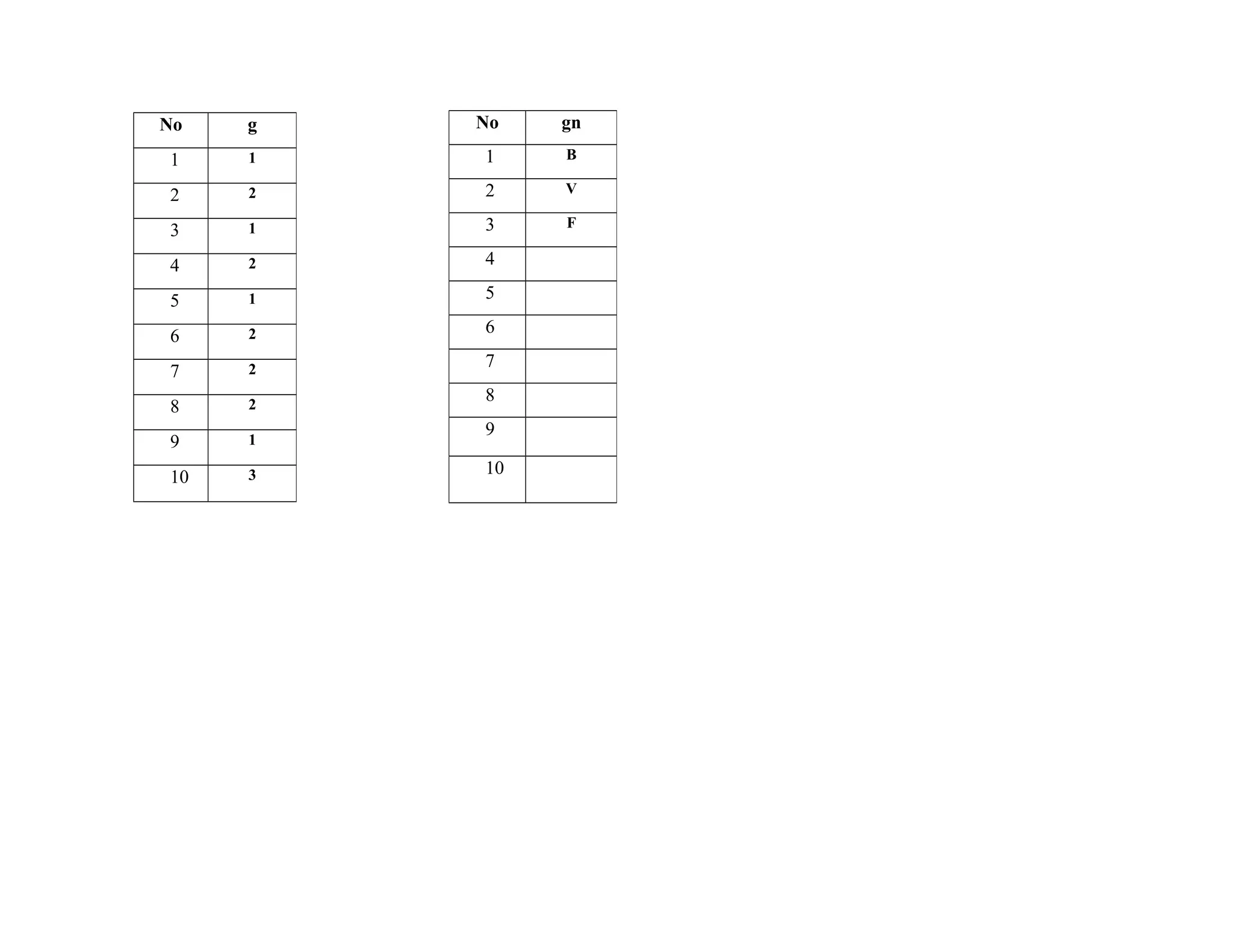
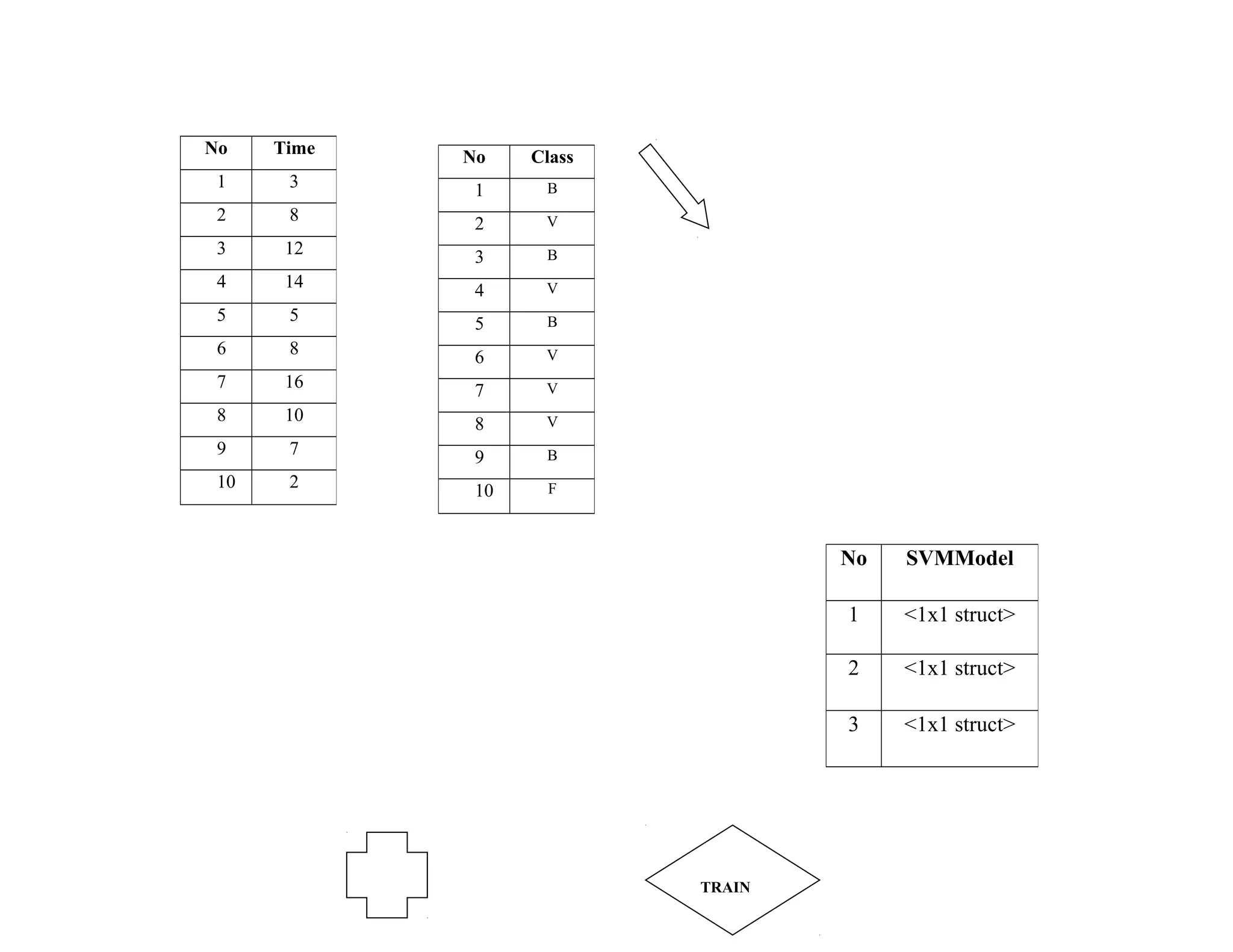
7. Step 2: After importing time and class to Matlab which converts Class into index vector because Class is a cell vector of strings; or a
character matrix with each row representing a group label.
[G,GN]=grp2idx(Class) creates an index vector G from the grouping variable Class.
Class can be a categorical, numeric, or logical vector; a cell vector of strings; or a character matrix with each row representing a group label.
After converting into index vector, the result G is a vector taking integer values from 1 up to the number K of distinct groups and GN
is a cell array of strings representing group labels. GN (G) reproduces Class.
In variable G we can see that there are three different digits 1, 2 and 3.
1 indicates Busy, 2 indicate Very Busy and 3 indicate Free class.
Table 3: Variable G and Gn after converting Class into index vector

8. No g
1 1
2 2
3 1
4 2
5 1
6 2
7 2
8 2
9 1
10 3
No gn
1 B
2 V
3 F
4
5
6
7
8
9
10

9. Step 3: After preparing original data the next task is to splitting dataset for training and testing. In dataset a training set is
implemented to build up a model. Data points in the training set are excluded from testing set or validation set. On the other hand,
testing set or validation set is used to validate the model built.
Usually a dataset is divided into a training set and validation set in each iteration.

10. No Time
1 3
2 8
3 12
4 14
5 5
6 8
7 16
8 10
9 7
10 2
No Class
1 B
2 V
3 B
4 V
5 B
6 V
7 V
8 V
9 B
10 F
No SVMModel
1 <1x1 struct>
2 <1x1 struct>
3 <1x1 struct>
TRAIN

11. Step 4: After training we will get a model and this model along with testing set will be used for classification using multi class SVM.
Figure 3: Time and Velocity Class used as Training Data

12. Field Value Minimum Maximum
Support Vectors <2059x1 double> 1 52
Alpha <2059x1 double> -0.1554 0.2806
Bias -0.68867509 -0.6887 -0.6887
Kernel Function @rbf_kernel
Kernel Function
Args
<1x1 cell>
Group Names <3654x1 double> 1 2
Support Vector
Indices
<2059x1 double> 1 3651
Scale Data [ ]
Figure Handles [ ]
No SVMModel
1 <1x1 struct>
2 <1x1 struct>
3 <1x1 struct>
Field Value Minimu
m
Maximum
Support Vectors <440x1 double> 1 52
Alpha <440x1 double> -0.7778 0.1148
Bias 0.779995289101020 0.7800 0.7800
Kernel Function @rbf_kernel
Kernel Function Args <1x1 cell>
Group Names <2699x1 double> 2 3
Support Vector
Indices
<440x1 double> 1 2683
Scale Data [ ]
Figure Handles [ ]

13. Step 5: After Classification using Multiclass Support Vector Machine I have used support vectors from each binary classification and
applied weighted moving average method (WMA) with a new equation.
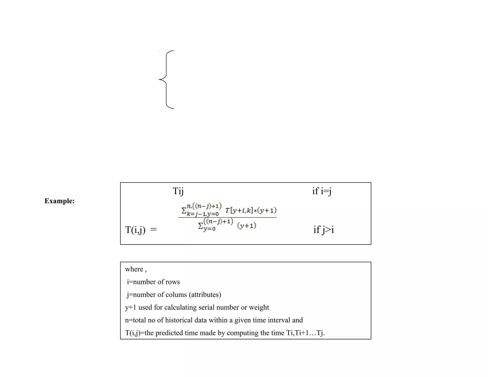
Weighted Moving average (WMA): In this proposed methods we can predict travel time by analyzing the historical travel time data.
As for example, a vehicle enters on a particular road segment at 10:00 AM and wants to predict travel time. For that reason, we need
to accumulate all historical travel time data for that road segment during 10:00 AM. Let t = t1, t2, ........tn be the historical travel time
data for any road segment where n is the total number of historical data within a given time interval. For travel time prediction
problem, I pick as my sub-problems the problem of determining the time prediction of ti , ti+1,........t j for 1 ≤ i ≤ j ≤ n . Let T[i, j] be
the predicted time made by computing the time ti , ti+1,........t j ; for the full problem, the predicted time to compute t1, t2 ,........tn
would thus be T [1, n].
Weighted moving average can be mathematically described by following formula:
Field Value Minimum Maximum
Support Vectors <660x1 double> 1 26
Alpha <660x1 double> -0.4752 0.1267
Bias 0.7203309399863
15
0.7203 0.7203
Kernel Function @rbf_kernel
Kernel Function
Args
<1x1 cell>
Group Names <1649x1 double> 1 3
Support Vector
Indices
<660x1 double> 1 1645
Scale Data [ ]
Figure
Handles
[ ]
Figure 4: Result of one verses one classification

14. Example:
Tij if i=j
T(i,j) = if j>i
where ,
i=number of rows
j=number of colums (attributes)
y+1 used for calculating serial number or weight
n=total no of historical data within a given time interval and
T(i,j)=the predicted time made by computing the time Ti,Ti+1…Tj.

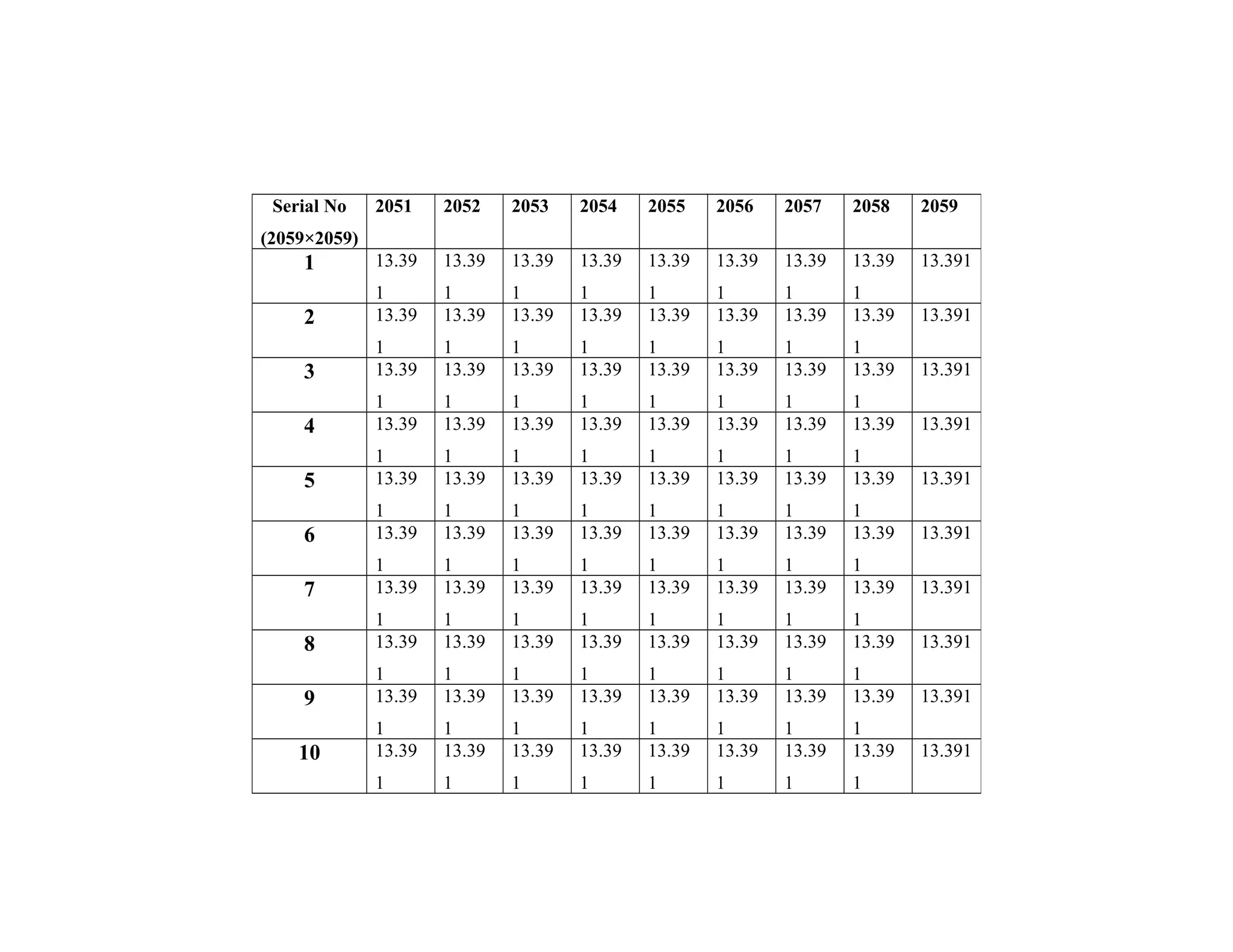
15. The T table is used for storing the value of T [ i, j ]. By using the equation of weighted moving average we can calculate the first value
.
=3.467
In this way the value in T[1,3] can be found by calculating weighted moving average of T[1, 2], T[2, 3], T[3,4] and T[4, 5] where
weight for them will be 1, 2, 3 and 4 respectively. Using the proposed method the value of T[1,5] will be the final predicted time.
After using weighted moving average, the predicted travel time would be 2.879.
T[i , j]
Serial No
(5×5)
1 2 3 4 5
1 5 3.4667 3.0233 2.9001
9
2.8790
2 0 3 3.3000 2.9389 2.8685
3 0 0 5 3.1666
7
2.8333
4 0 0 0 4 2.6667
5 0 0 0 0 2
Serial No
(1×5)
1 2 3 4 5
1 5 3 5 4 2
Figure 5: T table for proposed method (Weighted moving Average Method)

16. Serial No
(2059×2059)
2051 2052 2053 2054 2055 2056 2057 2058 2059
1 13.39
1
13.39
1
13.39
1
13.39
1
13.39
1
13.39
1
13.39
1
13.39
1
13.391
2 13.39
1
13.39
1
13.39
1
13.39
1
13.39
1
13.39
1
13.39
1
13.39
1
13.391
3 13.39
1
13.39
1
13.39
1
13.39
1
13.39
1
13.39
1
13.39
1
13.39
1
13.391
4 13.39
1
13.39
1
13.39
1
13.39
1
13.39
1
13.39
1
13.39
1
13.39
1
13.391
5 13.39
1
13.39
1
13.39
1
13.39
1
13.39
1
13.39
1
13.39
1
13.39
1
13.391
6 13.39
1
13.39
1
13.39
1
13.39
1
13.39
1
13.39
1
13.39
1
13.39
1
13.391
7 13.39
1
13.39
1
13.39
1
13.39
1
13.39
1
13.39
1
13.39
1
13.39
1
13.391
8 13.39
1
13.39
1
13.39
1
13.39
1
13.39
1
13.39
1
13.39
1
13.39
1
13.391
9 13.39
1
13.39
1
13.39
1
13.39
1
13.39
1
13.39
1
13.39
1
13.39
1
13.391
10 13.39
1
13.39
1
13.39
1
13.39
1
13.39
1
13.39
1
13.39
1
13.39
1
13.391

17. Figure 6: prediction of travel time for Busy and Very Busy class is 13.391 where minimum
value is 1 and maximum value is 52

18. Serial No
(660×660)
652 653 654 655 656 657 658 659 660
1 2.409 2.409 2.409 2.409 2.409 2.409 2.409 2.409 2.409
2 2.409 2.409 2.409 2.409 2.409 2.409 2.409 2.409 2.409
3 2.409 2.409 2.409 2.409 2.409 2.409 2.409 2.409 2.409
4 2.409 2.409 2.409 2.409 2.409 2.409 2.409 2.409 2.409
5 2.409 2.409 2.409 2.409 2.409 2.409 2.409 2.409 2.409
6 2.409 2.409 2.409 2.409 2.409 2.409 2.409 2.409 2.409
7 2.409 2.409 2.409 2.409 2.409 2.409 2.409 2.409 2.409
8 2.409 2.409 2.409 2.409 2.409 2.409 2.409 2.409 2.409
9 2.409 2.409 2.409 2.409 2.409 2.409 2.409 2.409 2.409
10 2.409 2.409 2.409 2.409 2.409 2.409 2.409 2.409 2.409
Figure 7: Prediction of Travel Time for Busy and Free class is 2.409 where minimum
value is 1 and maximum value is 52

19. Serial No
(440×440)
432 433 434 435 436 437 438 439 440
1 6.458 6.458 6.458 6.458 6.458 6.458 6.458 6.458 6.458
2 6.458 6.458 6.458 6.458 6.458 6.458 6.458 6.458 6.458
3 6.458 6.458 6.458 6.458 6.458 6.458 6.458 6.458 6.458
4 6.458 6.458 6.458 6.458 6.458 6.458 6.458 6.458 6.458
5 6.458 6.458 6.458 6.458 6.458 6.458 6.458 6.458 6.458
6 6.458 6.458 6.458 6.458 6.458 6.458 6.458 6.458 6.458
7 6.458 6.458 6.458 6.458 6.458 6.458 6.458 6.458 6.458
8 6.458 6.458 6.458 6.458 6.458 6.458 6.458 6.458 6.458
9 6.458 6.458 6.458 6.458 6.458 6.458 6.458 6.458 6.458
10 6.458 6.458 6.458 6.458 6.458 6.458 6.458 6.458 6.458

20. So the average travel time is (13.391+2.409+6.458)/3=7.419sec.
Result Analysis: A real data set is used in this study, which was collected by PNU (Pusan National University) trajectory data
generator. This generator is based on real traffic situation in Pusan City, South Korea. For building PNU generator, they collected real
traffic data by using GPS sensor. From this data, traffic pattern of Pusan city was extracted. And according to traffic pattern, generator
simulates and generates trajectory data, which is almost same as real data. The period of real traffic data covers both weekdays and
weekends, and both peak hours and non-peak hours. This should adequately reflect real traffic situations. By using this generator,
167,669 trajectories are generated.
Every trajectory may be composed of several road segments. This data organization format sufficiently reflects real traffic situations.
For computing easily and efficiently and accurate evaluation of performance of the algorithms, data is divided into two categories,
namely training data and test data sets. 365 days traffic data are used as training data set and 30 days traffic data are used as testing
dataset. Testing data sets are chronologically after 365 days data used for training. Data from 365 training days are used for fitting the
model. However, 30 days test data are used to measure prediction performance for all methods.
Figure 8: Prediction of Travel Time for Very Busy and Free class is 6.458 where
minimum value is 1 and maximum value is 52

21. The prediction error indices, Mean Absolute Relative Error (MARE) are used to compare the accuracy among all prediction methods.
MARE is the simplest and well-known method for measuring overall error in travel time prediction. MARE measures the magnitude
of the relative error over the desired time range. The MARE is measured by the following formula:
where, x(t) is the observation value, x* (t) is the predicted value and N is the number of samples. In experimental evaluation, proposed
methods are tested against other predictors like Chain Average (CA), Successive Moving Average (SMA) and Artificial Neural
Network (ANN). Prediction errors of all predictors from 8 AM to 5 PM are examined. There are 10 test cases evaluated between 8
AM and 5 PM.
The line chart shown in Fig.4.1 illustrates relative performance of all travel time predictors.

22. From the overall point of view, proposed method performs much better than CA, SMA, and ANN method. In case of SVM & WMA
method, it is shown that seven test cases exhibit errors less than or equal to 0.40. At 10.00 AM, 9.00 AM and 5.00 PM our method
SVM &WMA predicted more accurately than others and datasets of those period included uncertain data. By contrary Support Vector
Machine and Weighted Moving Average (SVM, WMA), Artificial Neural Network (ANN), Successive Moving Average (SMA) and
Chain Average (CA) outperform our method in one, two and one cases respectively but that are slight differences.
Summarized result of MARE for different travel time predictors are shown in Fig. 4.2.MARE of SVM &WMA, CA, SMA and ANN
are 3.13, 3.92, 4.07 and 4.82 respectively.
Thus, our proposed method reduces MARE from CA, SMA and ANN method by 19%, 23% and 40% respectively.
Conclusion: This research explored mainly the use of support vector machine and weighted moving average method for travel time
prediction of transit vehicles under traffic conditions given GPS data. I have proposed a method for travel time prediction by using
real time traffic data from PNU trajectory generator. This work focuses on travel time prediction in road network for Advanced
Traveller Information System (ATIS).
The requirements for such an ATIS system include real-time data collection and methodologies for quick travel time prediction.
Before the SVM development, ANN spatial and temporal correlations between travel times, running times and dwell times were
investigated. The common variations in travel times, i.e. systematic and random variations have also been studied.

23. The research used GPS data which isn’t quite a new data collection scheme in the area and an algorithm based on SVM and WMA has
been developed for predicting the travel time of transit vehicles between any two road segments under consideration. As one might
expect, the traffic conditions in developing countries are different with heterogeneity lack of lane discipline. Therefore, the prediction
algorithm needs more care during development as compared to short-term travel time prediction that used homogeneous data in most
previous reported studies on. The lack of historic data and permanent data collection schemes add to the difficulties.
This paper focuses on travel time prediction in road network for Advanced Traveller Information System (ATIS). In this paper, we
have developed two methods for predicting travel time by using real traffic data from Pusan National University (PNU) trajectory
generator. Compared to the other methods, simulation results suggest that proposed methods provide a more precise prediction in most
test cases.