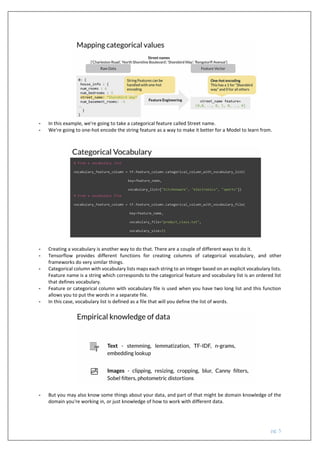
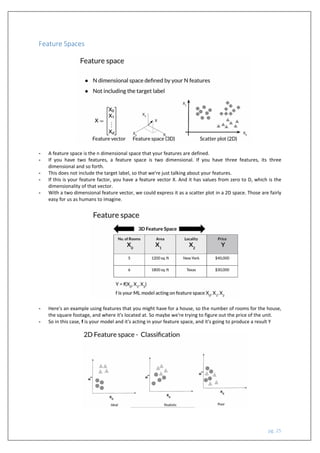
The document outlines a course on machine learning engineering focused on data lifecycle in production, emphasizing the importance of data pipelines, feature engineering, and production-ready skills. It covers essential topics like preprocessing operations, dimensionality reduction, and techniques for ensuring consistent transformations between training and serving models. The course aims to equip learners with practical knowledge to effectively handle large-scale data and improve the predictive power of machine learning models.


![pg. 11
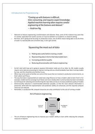
Feature Crosses
- What are Feature crosses? Well, they combine multiple features together into a new feature. That's
fundamentally what a feature across.
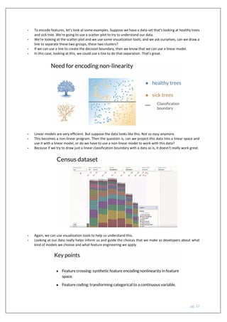
- It encodes non-linearity in the feature space, or encodes the same information with fewer features.
- We can create many different kinds of feature crosses and it really depends on our data.
- It requires a little bit of imagination to look for ways to try to do that, to combine the features that we have.
- For example, if we have numerical features, we could multiply two features [A x B] and produce one feature
that has an expression of those two features.
- If we have 5 features, we could multiply them all together if there are numerical features and then end up
with one feature instead of say five.
- We can also take categorical features or even numerical features and combine them in ways that make a
semantic sense.
- Taking the day of the week and hour, if those are two different features that we have, putting those together,
we can express that as the hour of the week and we have the same information in one feature.](https://image.slidesharecdn.com/week2-featureengineeringtransformationandselection-210918180724/85/Machine-Learning-Data-Life-Cycle-in-Production-Week-2-feature-engineering-transformation-and-selection-11-320.jpg)


![[DSC Europe 25] Andrzej Kowalczyk - AI - how to start small and grow in the f...](https://cdn.slidesharecdn.com/ss_thumbnails/oy1zmo94qv6vpcqjvno2-andrzej-kowalczyk-ai-how-to-start-small-and-grow-in-the-future-1-260119121559-cf093b23-thumbnail.jpg?width=640&height=640&fit=bounds)
![[DSC Europe 25] Mikhail Rozhkov - AI Product Canvas: From Business Goals to T...](https://cdn.slidesharecdn.com/ss_thumbnails/d53doddtpgfqivmzqel6-mikhail-rozhkov-ai-product-canvas-v1-260121115910-9dd517a7-thumbnail.jpg?width=640&height=640&fit=bounds)


![[DSC Europe 25] Borko Kozomora - Optimizing business workflows with advances ...](https://cdn.slidesharecdn.com/ss_thumbnails/hbgekyb0txw0xpo4yfml-borko-kozomora-leading-ai-transformation-260122103838-cc29ee38-thumbnail.jpg?width=640&height=640&fit=bounds)
![[DSC Europe 25] Paula Garcia Esteban -Building the Future: The Role of Data S...](https://cdn.slidesharecdn.com/ss_thumbnails/9ld1r1bsqpwve8qfvphy-paula-garcia-esteban-building-the-future-260122103838-4171f5cb-thumbnail.jpg?width=640&height=640&fit=bounds)

![[DSC Europe 25] Bojan Banjac - AI is always right when it comes to the matter...](https://cdn.slidesharecdn.com/ss_thumbnails/syoxtqierpydwxm5srcb-4-bojan-banjac-ai-is-always-right-when-it-comes-to-the-matters-of-taste-260119101519-694ee7d7-thumbnail.jpg?width=640&height=640&fit=bounds)
![[DSC Europe 25] Milovan Jovicic - Beyond AI's Reach: The Enduring Value of Ev...](https://cdn.slidesharecdn.com/ss_thumbnails/pyeij0hurgwq5jugmtnv-2-milovan-jovicic-beyond-ais-reach-the-enduring-value-of-evergreen-design-v2-260120105856-d6ee57e5-thumbnail.jpg?width=640&height=640&fit=bounds)


