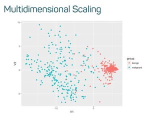
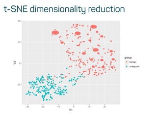
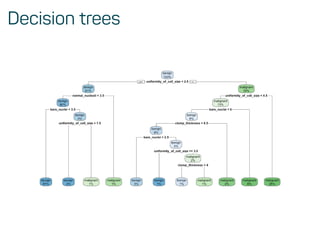
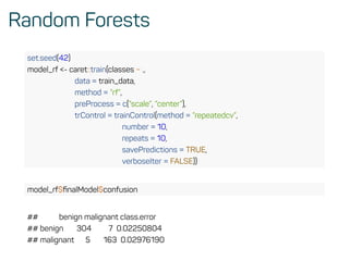
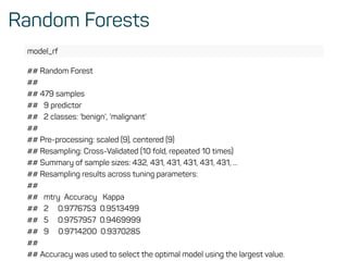
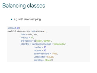
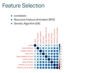
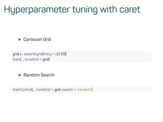
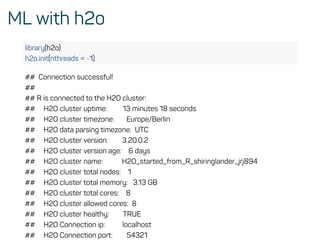
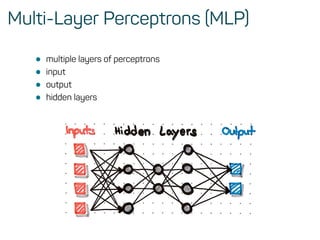
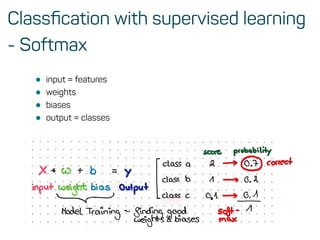
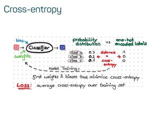
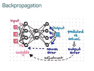
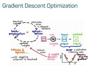
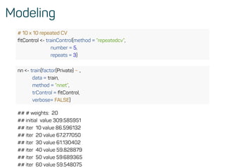
The document is a workshop guide on machine learning using R, covering essential topics such as data preparation, the caret and h2o packages, and neural networks. It includes practical examples and code snippets for various ML techniques like decision trees, random forests, and hyperparameter tuning. The guide is aimed at practitioners who wish to understand and apply machine learning concepts effectively.

1. Introduction to Machine
Learning with R
Dr. Shirin Glander
codecentric AG
28.06.2018

2. Table of Contents
About me & this workshop
Getting started
Machine Learning
How to prepare your data for ML
ML with caret
ML with h2o
Deep Dive into Neural Networks
How do Neural Nets learn?
Training neural nets in R

3. About me & this workshop

4. How I ended up here

5. About this workshop
Machine Learning with the caret package
• data prep
• missingness
• decision trees
• random forests
• gradient boosting
• feature selection
• hyperparameter tuning
• plotting
Machine Learning with the h2o package
• hyperparameter tuning

6. If there is still time…
Deep Dive into Neural Networks
• what are neural nets and what makes them special?
• how do neural nets learn?
• how to train neural nets with caret

7. Workshop material
Scripts and code
https://gitlab.com/ShirinG/intro_to_ml_workshop
• Code-Through: intro_to_ml.html*
• Slides: slides/intro_to_ml_slides.pdf
• Datasets: datasets/

8. Why use R
• open-source, cross-platform
• established language (there are lots and lots of packages)
• high quality packages with proper documentation (CRAN)
• graphics capabilities - ggplot2!!!
• RStudio + R Markdown!!
• community support!

9. Getting started

10. R + RStudio - Best practices
• Step 1) create a new project

11. R + RStudio - Best practices
• Step 2) create a new R Markdown document

12. Machine Learning

13. Machine Learning (ML) overview

14. A general workflow
• Input data
• Data preprocessing
• Training, validation and test split
• Modeling
• Predictions and Evaluations

15. How to prepare your data for ML

16. Reading in data
Breast Cancer Wisconsin (Diagnostic) Dataset
library(tidyverse) # for tidy data analysis
bc_data <- readr::read_delim(”../datasets/breast-cancer-wisconsin.data.txt”,
delim = ”,”,
col_names = c(”sample_code_number”,
”clump_thickness”,
”uniformity_of_cell_size”,
”uniformity_of_cell_shape”,
”marginal_adhesion”,
”single_epithelial_cell_size”,
”bare_nuclei”,
”bland_chromatin”,
”normal_nucleoli”,
”mitosis”,
”classes”)) %>%
mutate(bare_nuclei = as.numeric(bare_nuclei),
classes = ifelse(classes == ”2”, ”benign”,
ifelse(classes == ”4”, ”malignant”, NA)))

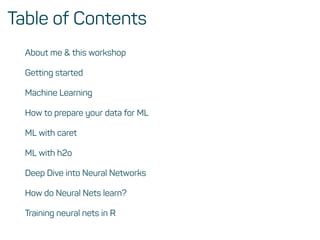
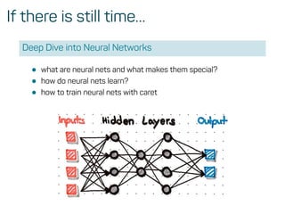
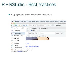
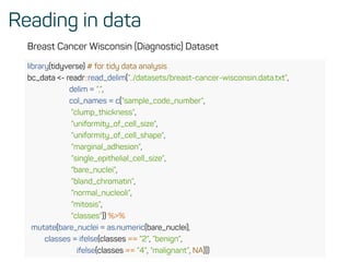
17. Missingness
mice::md.pattern(bc_data, plot = FALSE)
## sample_code_number clump_thickness uniformity_of_cell_size
## 683 1 1 1
## 16 1 1 1
## 0 0 0
## uniformity_of_cell_shape marginal_adhesion single_epithelial_cell_size
## 683 1 1 1
## 16 1 1 1
## 0 0 0
## bland_chromatin normal_nucleoli mitosis classes bare_nuclei
## 683 1 1 1 1 1 0
## 16 1 1 1 1 0 1
## 0 0 0 0 16 16
bc_data <- bc_data[complete.cases(bc_data), ] %>% .[, c(11, 2:10)]
• or impute with the mice package

18. Response variable for classification
ggplot(bc_data, aes(x = classes, fill = classes)) + geom_bar()
0
100
200
300
400
benign malignant
classes
count
classes
benign
malignant
• Consider balancing of response classes!!!

19. Feature correlation graphs

20. Principal Component Analysis

21. Multidimensional Scaling

22. t-SNE dimensionality reduction

23. ML with caret

24. Training, validation & testing
• balance between generalization and specificity
• to prevent over-fitting!
• validation sets or cross-validation

25. Training, validation & testing
• balance between generalization and specificity
• to prevent over-fitting!
• validation sets or cross-validation

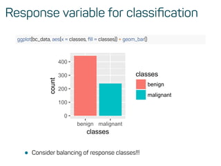
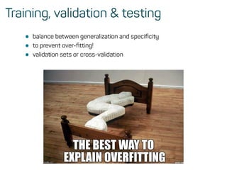
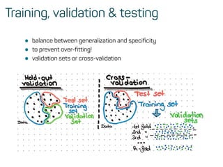
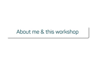
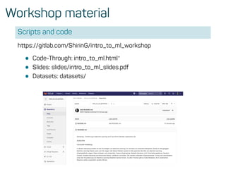
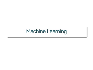
26. Training, validation and test data
library(caret)
set.seed(42)
index <- createDataPartition(bc_data$classes, p = 0.7, list = FALSE)
train_data <- bc_data[index, ]
test_data <- bc_data[-index, ]
• the main function in caret
?caret::train
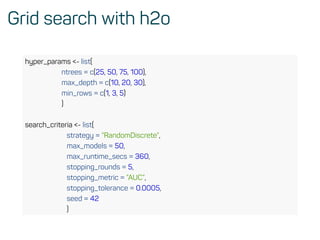
This function sets up a grid of tuning parameters for a
number of classification and regression routines, fits each
model and calculates a resampling based performance
measure.

27. Decision trees

28. Random Forests
set.seed(42)
model_rf <- caret::train(classes ~ .,
data = train_data,
method = ”rf”,
preProcess = c(”scale”, ”center”),
trControl = trainControl(method = ”repeatedcv”,
number = 10,
repeats = 10,
savePredictions = TRUE,
verboseIter = FALSE))
model_rf$finalModel$confusion
## benign malignant class.error
## benign 304 7 0.02250804
## malignant 5 163 0.02976190

29. Random Forests
model_rf
## Random Forest
##
## 479 samples
## 9 predictor
## 2 classes: 'benign', 'malignant'
##
## Pre-processing: scaled (9), centered (9)
## Resampling: Cross-Validated (10 fold, repeated 10 times)
## Summary of sample sizes: 432, 431, 431, 431, 431, 431, ...
## Resampling results across tuning parameters:
##
## mtry Accuracy Kappa
## 2 0.9776753 0.9513499
## 5 0.9757957 0.9469999
## 9 0.9714200 0.9370285
##
## Accuracy was used to select the optimal model using the largest value.

30. Balancing classes
• e.g. with downsampling
set.seed(42)
model_rf_down <- caret::train(classes ~ .,
data = train_data,
method = ”rf”,
preProcess = c(”scale”, ”center”),
trControl = trainControl(method = ”repeatedcv”,
number = 10,
repeats = 10,
savePredictions = TRUE,
verboseIter = FALSE,
sampling = ”down”))

31. Feature Importance
importance <- varImp(model_rf, scale = TRUE)
plot(importance)
Importance
mitosis
marginal_adhesion
clump_thickness
single_epithelial_cell_size
normal_nucleoli
bland_chromatin
bare_nuclei
uniformity_of_cell_shape
uniformity_of_cell_size
0 20 40 60 80 100

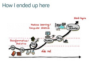
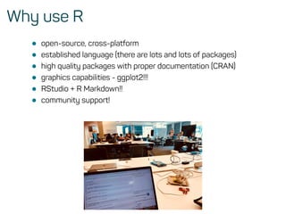
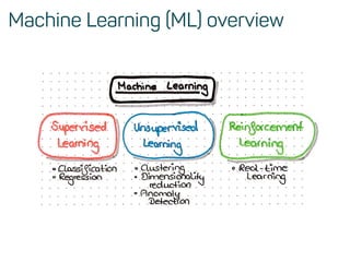
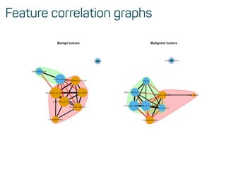
32. Predictions on test data
confusionMatrix(predict(model_rf, test_data), as.factor(test_data$classes))
## Confusion Matrix and Statistics
##
## Reference
## Prediction benign malignant
## benign 128 4
## malignant 5 67
##
## Accuracy : 0.9559
## 95% CI : (0.9179, 0.9796)
## No Information Rate : 0.652
## P-Value [Acc > NIR] : <2e-16
##
## Kappa : 0.9031
## Mcnemar's Test P-Value : 1
##
## Sensitivity : 0.9624
## Specificity : 0.9437

33. Extreme gradient boosting trees
• available models in caret: https://topepo.github.io/caret
set.seed(42)
model_xgb <- caret::train(classes ~ .,
data = train_data,
method = ”xgbTree”,
preProcess = c(”scale”, ”center”),
trControl = trainControl(method = ”repeatedcv”,
number = 10,
repeats = 10,
savePredictions = TRUE,
verboseIter = FALSE))

34. Extreme gradient boosting trees
model_xgb
## eXtreme Gradient Boosting
##
## 479 samples
## 9 predictor
## 2 classes: 'benign', 'malignant'
##
## Pre-processing: scaled (9), centered (9)
## Resampling: Cross-Validated (10 fold, repeated 10 times)
## Summary of sample sizes: 432, 431, 431, 431, 431, 431, ...
## Resampling results across tuning parameters:
##
## eta max_depth colsample_bytree subsample nrounds Accuracy
## 0.3 1 0.6 0.50 50 0.9567788
## 0.3 1 0.6 0.50 100 0.9544912
## 0.3 1 0.6 0.50 150 0.9513572
## 0.3 1 0.6 0.75 50 0.9576164
## 0.3 1 0.6 0.75 100 0.9536448

35. Feature Selection
• correlation
• Recursive Feature elimination (RFE)
• Genetic Algorithm (GA)

36. Hyperparameter tuning with caret
• Cartesian Grid
grid <- expand.grid(mtry = c(1:10))
train(..., tuneGrid = grid)
• Random Search
trainControl(..., tuneGrid = grid, search = ”random”)

37. ML with h2o

38. ML with h2o
library(h2o)
h2o.init(nthreads = -1)
## Connection successful!
##
## R is connected to the H2O cluster:
## H2O cluster uptime: 13 minutes 18 seconds
## H2O cluster timezone: Europe/Berlin
## H2O data parsing timezone: UTC
## H2O cluster version: 3.20.0.2
## H2O cluster version age: 6 days
## H2O cluster name: H2O_started_from_R_shiringlander_jrj894
## H2O cluster total nodes: 1
## H2O cluster total memory: 3.13 GB
## H2O cluster total cores: 8
## H2O cluster allowed cores: 8
## H2O cluster healthy: TRUE
## H2O Connection ip: localhost
## H2O Connection port: 54321

39. Grid search with h2o
hyper_params <- list(
ntrees = c(25, 50, 75, 100),
max_depth = c(10, 20, 30),
min_rows = c(1, 3, 5)
)
search_criteria <- list(
strategy = ”RandomDiscrete”,
max_models = 50,
max_runtime_secs = 360,
stopping_rounds = 5,
stopping_metric = ”AUC”,
stopping_tolerance = 0.0005,
seed = 42
)

40. Grid search with h2o

41. Evaluate model performance
• Variable importance
h2o.varimp_plot(rf_model)
mitosis
marginal_adhesion
clump_thickness
normal_nucleoli
single_epithelial_cell_size
bland_chromatin
bare_nuclei
uniformity_of_cell_shape
uniformity_of_cell_size
Variable Importance: DRF
.0
.2
.4
.6
.8
.0

42. Evaluate model performance
h2o.mean_per_class_error(rf_model, train = TRUE, valid = TRUE, xval = TRUE)
## train valid xval
## 0.02196246 0.02343750 0.02515735
h2o.confusionMatrix(rf_model, valid = TRUE)
## Confusion Matrix (vertical: actual; across: predicted) for max f1 @ threshold = 0.5333333
## benign malignant Error Rate
## benign 61 3 0.046875 =3/64
## malignant 0 38 0.000000 =0/38
## Totals 61 41 0.029412 =3/102

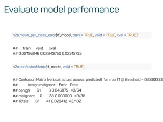
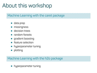
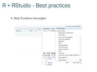
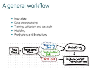
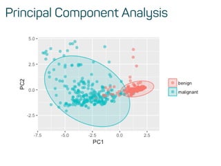
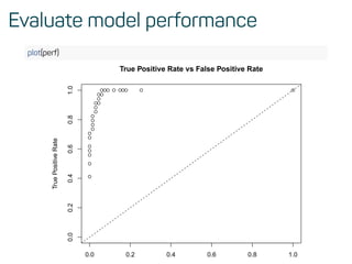
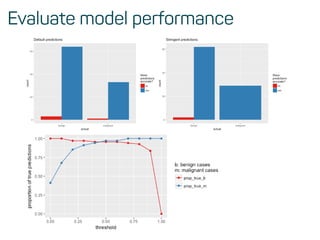
43. Evaluate model performance
perf <- h2o.performance(rf_model, test)
h2o.logloss(perf)
## [1] 0.1072519
h2o.mse(perf)
## [1] 0.03258482
h2o.auc(perf)
## [1] 0.9916594

44. Evaluate model performance
plot(perf)
0.0 0.2 0.4 0.6 0.8 1.0
0.00.20.40.60.81.0 True Positive Rate vs False Positive Rate
TruePositiveRate

45. Evaluate model performance

46. Deep Dive into Neural Networks

47. Introduction to Neural Networks (NN)
• machine learning framework
• attempts to mimic the learning pattern of the brain (biological
neural networks)
• Artificial Neural Networks = ANNs

48. Perceptrons
• Input (multiplied by weight)
• Bias
• Activation function
• Output

49. Multi-Layer Perceptrons (MLP)
• multiple layers of perceptrons
• input
• output
• hidden layers

50. How do Neural Nets learn?

51. Classfication with supervised learning
- Softmax
• input = features
• weights
• biases
• output = classes

52. Cross-entropy

53. Backpropagation

54. Gradient Descent Optimization

55. Training neural nets in R

56. Features & data preprocessing
library(ISLR)
print(head(College))
Private Apps Accept Enroll Top10perc Top25perc F.Undergrad P.Undergrad Outstate Room.Board Books Personal PhD Terminal S.F.Ratio perc.alumni Expend Grad.Rate
Abilene Christian University Yes 1660.00 1232.00 721.00 23.00 52.00 2885.00 537.00 7440.00 3300.00 450.00 2200.00 70.00 78.00 18.10 12.00 7041.00 60.00
Adelphi University Yes 2186.00 1924.00 512.00 16.00 29.00 2683.00 1227.00 12280.00 6450.00 750.00 1500.00 29.00 30.00 12.20 16.00 10527.00 56.00
Adrian College Yes 1428.00 1097.00 336.00 22.00 50.00 1036.00 99.00 11250.00 3750.00 400.00 1165.00 53.00 66.00 12.90 30.00 8735.00 54.00
Agnes Scott College Yes 417.00 349.00 137.00 60.00 89.00 510.00 63.00 12960.00 5450.00 450.00 875.00 92.00 97.00 7.70 37.00 19016.00 59.00
Alaska Pacific University Yes 193.00 146.00 55.00 16.00 44.00 249.00 869.00 7560.00 4120.00 800.00 1500.00 76.00 72.00 11.90 2.00 10922.00 15.00
Albertson College Yes 587.00 479.00 158.00 38.00 62.00 678.00 41.00 13500.00 3335.00 500.00 675.00 67.00 73.00 9.40 11.00 9727.00 55.00
# Create vector of column max and min values
maxs <- apply(College[, 2:18], 2, max)
mins <- apply(College[, 2:18], 2, min)
# Use scale() and convert the resulting matrix to a data frame
scaled.data <- as.data.frame(scale(College[,2:18],
center = mins,
scale = maxs - mins))

57. Train and test split
# Convert column Private from Yes/No to 1/0
Private = as.numeric(College$Private)-1
data = cbind(Private,scaled.data)
library(caret)
set.seed(42)
# Create split
idx <- createDataPartition(data$Private, p = .75, list = FALSE)
train <- data[idx, ]
test <- data[-idx, ]

58. Modeling
# 10 x 10 repeated CV
fitControl <- trainControl(method = ”repeatedcv”,
number = 5,
repeats = 3)
nn <- train(factor(Private) ~ .,
data = train,
method = ”nnet”,
trControl = fitControl,
verbose= FALSE)
## # weights: 20
## initial value 309.585951
## iter 10 value 86.596132
## iter 20 value 67.277050
## iter 30 value 61.130402
## iter 40 value 59.828879
## iter 50 value 59.689365
## iter 60 value 59.548075

59. Predictions and Evaluations
# Compute predictions on test set
predicted.nn.values <- predict(nn, test[2:18])
# print results
print(head(predicted.nn.values, 3))
## [1] 1 1 1
## Levels: 0 1
table(test$Private, predicted.nn.values)
## predicted.nn.values
## 0 1
## 0 47 3
## 1 4 140

60. Thank you!
… and stay in contact
• @ShirinGlander
• www.shirin-glander.de
• www.codecentric.de
• https://www.youtube.com/codecentricAI