Download to read offline
![Bipolar disorder investigation using modified logistic ridge estimator
DOI: 10.9790/5728-11131215 www.iosrjournals.org 13 |Page
The collinearity problem can be addressed by the following existing methods: Variable Selection,
Ridge Regression, and Principal Component Analysis etc.
Ridge Regression
This procedure is used in combating collinearity in GLM using the correlation matrix, standardized
regression coefficient and by introducing the biasing constant C, into the normal equations of the standardized
regression model. The ridge regression procedure can be stated using the following normal equation Tikhonov
etal (1998),
γXY
β = γXX
,
whereγXY
is the matrix correlation of Y with X and γXY
is the matrix correlation of X. Adding the biasing
constantC to the normal equation, we
γXX
+ CΙ β
R
= (γXX
+ CΙ)−1
γXX
Several successive values of C are tried until the regression coefficient becomes stable.By Ordinary Least
Squares estimation, we consider the system Xβ = Y
II. Method
The Logistic Ridge Estimator
The modified logistic Ridge estimator derives from the Logistic Ridge estimator as an extension of the
logistic estimator. In logistic Ridge regression, a biasing constant is introduced into the information matrix in
order to overcome the problem of collinearity. Where collinearity exists among explanatory variables, the
ordinary logistic regression becomes inadequate because of singularity problems.
The logistic regression model is given by the log of an odd or logit of a response probability as follows
Logit μ = Log
μ
1−μ
= β0
+ β1
x1 + β2
x2 + … + βk
xk (1)
whereμ = 1 + exp −(β0
+ βk
t
k=1 xk)
−1
.The expression
μ
1−μ
is called an odd of a favorable outcome and it
is expressed as
μ
1−μ
= exp β0
+ βk
xk
t
k=1
Let μhijk
denote the response probability for the hth
sex status, ith
age category, jth
occupational status, and kth
Body Mass Index (BMI).The Logistic model is then written as
log
μhijk
1−μhijk
= β0
+ βk
Xhijk
t
k=1
Maximum Likelihood (McCullagh and Nelder (1972), Der and Everitt (2009)) is used to estimate the parameters
of the logistic model in equation (1).The log likelihood function for the logistic model is given as
L (β;y) = yii log μ β′
xi + 1 − yi log 1 − μ β′
xi ,
wherey′
= [y1, y2, … , yn] are the n observed values of the dichotomous response variable.However,
because of the singularity of the ordinary logistic model as earlier mentioned, the logistic Ridge regression is
used to estimate this parameter values.
In this work, collinearity has been established among the explanatory variables under study. It is to be
observed that the variables under investigation are both categorical and continuous. A test for collinearity using
standard errors of parameter estimates and condition numbers reveal the existence of collinearity among the
explanatory variables. Running the analysis using both the logistic estimator and the logistic Ridge estimator
separately, reveals that the Ridge estimator has smaller standard errors. The logistic Ridge estimator (Tikhonov
et al (1998)) is given as
β = X′
WX + θΙ −1
X′
Z, (2)
Where,θ is the Tikhonov constant, Ζ is the adjusted dependent variable, W is a weight matrix, and X is the
designed matrix.
The initial value of this constant is normally intelligently guessed. This constant can also be generalized as in
the case of Generalized Logistic Ridge regression. The components of W and Ζ are given respectively as
wi = miμi 1−μi
zi = ηi
+ y − μi
1
μi
1 − μi](https://image.slidesharecdn.com/c011131215-151123093800-lva1-app6892/75/Bipolar-Disorder-Investigation-Using-Modified-Logistic-Ridge-Estimator-2-2048.jpg)
![Bipolar disorder investigation using modified logistic ridge estimator
DOI: 10.9790/5728-11131215 www.iosrjournals.org 15 |Page
From this result, we can conclude that older men are more predisposed to bipolar disorder than their
female or younger counterparts.A further analysis uses odd ratios. This shows that the odd ratio of bipolar
disorder for females versus males at teaching level≥ 40years is 0.73 or 73:100 against the males. That of
females versus males at teaching level but <40years is 74:100.Again, the odds are against males. This again
supports the fact of the response probability stated above that men are more predisposed to bipolar disorder than
females.
Effective screening programs along with early identification and intervention are increasingly
important in today’s economic climate that places enormous emphasis health care costs and optimizing
employee productivity. Accurate and timely recognition of BD has the potential to reduce medical costs and
indirect costs due to work loss.
References
[1]. American Psychiatric Association (2001). Diagnostic and Statistical Manual of Mental Disorders (4th
ed.).Washington, DC:
TeRevision (DSM-IV-TR).
[2]. Benazzi, F. (2004).Inter-episode mood liability in mood disorders: residual symptom or natural course of illness? Psychiatry
ClinNeurosci.58(5):480-6.
[3]. Brook, A.R et al (2006). Incurring Greater Health care Costs; Risk Stratification of Employees with Bipolar Disorder.Journal of
Clinical Psychiatry, Vol.8 (1).
[4]. Der, G.&Everitt, S. (2009).A Handbook of Analysis usingSAS (3rd edition).Boca Raton: CRC Press,Champion and Hall.
[5]. Gnust, R.F (1984).Toward a Balanced Assessment of Collinearity Diagnostics. American Statistician.Vol.38, p. 79-82.
[6]. Huxley NA, Parikh SV, Baldessarini RJ.(2000) Effectiveness of psychosocial treatments in bipolar disorder: state of the evidence.
Harv Rev sychiatry.8(3):126–140.
[7]. Mason, G. (1987). Coping with Collinearity University of Manitoba Research Ltd. The Canadian Journal of Program Evaluation
[8]. McCullagh, P.&Nelder, J.A. (1992).Generalized Linear Models. Chapman and Hall, Madras.
[9]. Mental Health: A Report of the Surgeon General. U.S. Department of Health and Human Services, Substance Abuse and Mental
Health Services Administration, Center for Mental Health Services, National Institutes of Health, National Institute of Mental
Health. 1999
[10]. Motalskey, H. (2002).Multicollinearity in multiple Regression President, Graph pad Software ( hmotulsky @ graphpad.com).
[11]. Ogoke U.P, Nduka E.C, &NjaM.E (2013). A New Logistic Ridge Regression Estimator using ExponentiatedResponse
Function.Journal of Statistical and Econometric Method.Vol. 2 (4), p. 161-171.
[12]. Paykel E.S, Abbott R, Morriss R, Hayhurst H, Scott J.(2006), Sub-syndromal and syndromal symptoms in the longitudinal course of
bipolar disorder. Br J Psychiatry. 189:118-23
[13]. Sachs GS, Printz DJ, Kahn DA, Carpenter D, Docherty JP. (2000): Medication Treatment of Bipolar Disorder, The Expert
Consensus ) Guideline Series Postgrad Med. Apr;Spec No.:1–104.
[14]. Sachs G.S, Thase,M.E(2000). Bipolar disorder therapeutics:treatment. BiolPsychiatry.48 (6):573–581.
[15]. Tikhonov, A.N, Leonov, A.S, Yagola, A.G (1998): Non linear ill-posed problems, vol. 1, vol. 2 Chapman & Hall.
[16]. Weissfield&Sereika (1991): A Multicollinearity Diagnostic for Generalized Linear Models.](https://image.slidesharecdn.com/c011131215-151123093800-lva1-app6892/75/Bipolar-Disorder-Investigation-Using-Modified-Logistic-Ridge-Estimator-4-2048.jpg)

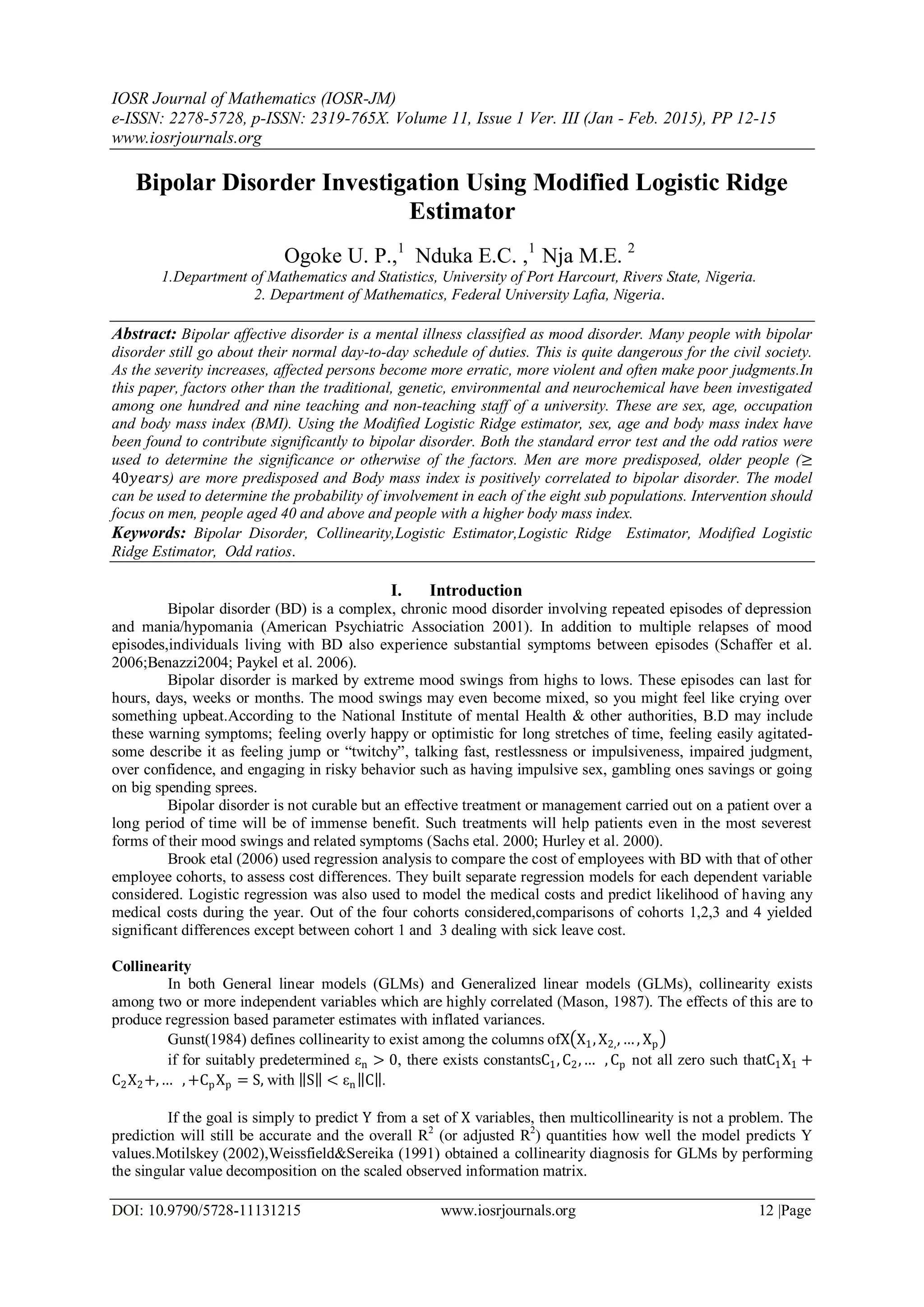
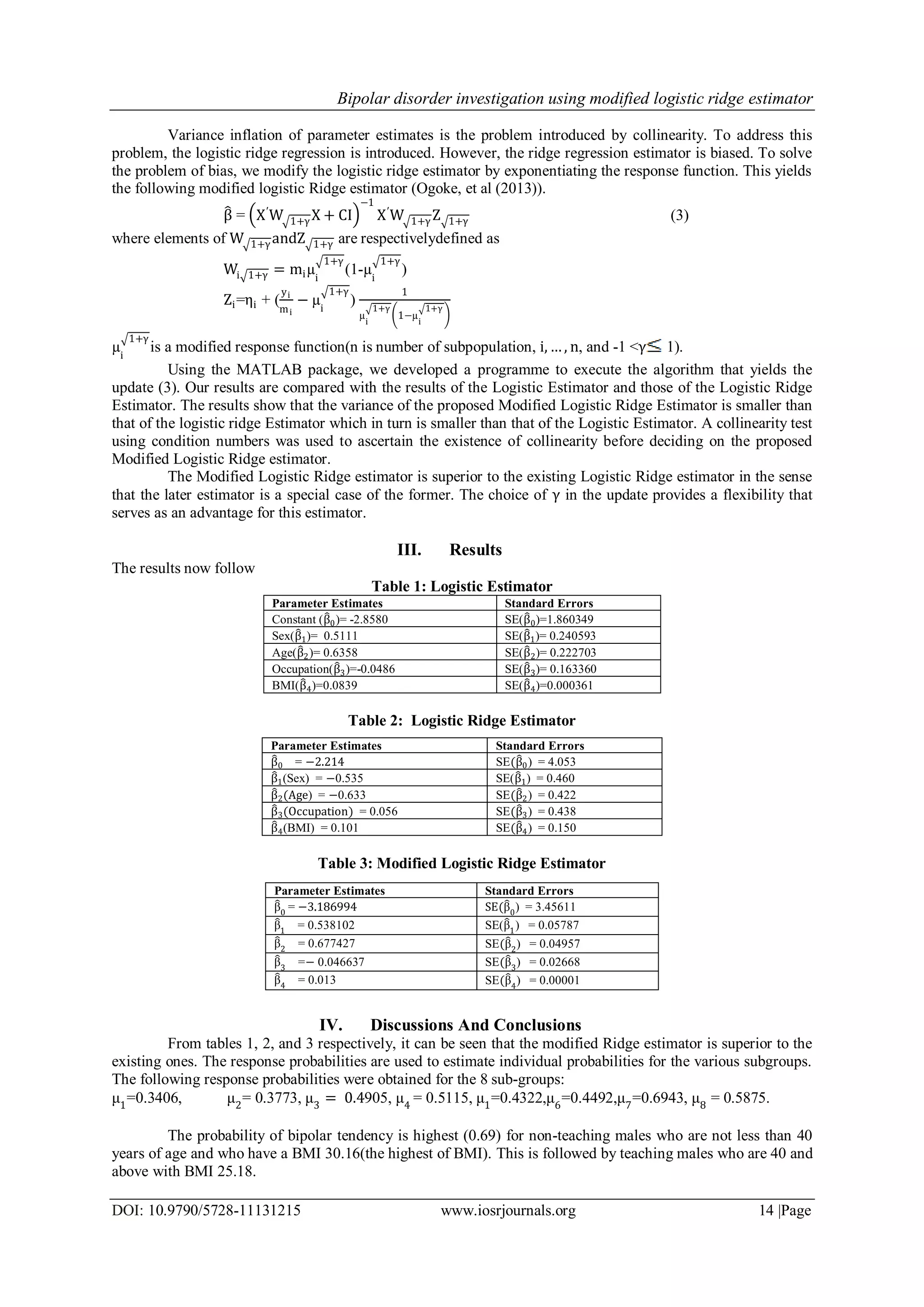
This study investigates factors contributing to bipolar disorder among 109 teaching and non-teaching university staff using a modified logistic ridge estimator. Sex, age, occupation, and body mass index were analyzed as factors beyond traditional genetic, environmental, and neurochemical factors. The modified logistic ridge estimator was found to have smaller standard errors than the standard logistic ridge estimator or logistic estimator. The results found that sex, age, and body mass index significantly contribute to bipolar disorder, with men and older adults (≥40 years) being more predisposed, and higher body mass index positively correlated with bipolar disorder. The probability of bipolar tendency was highest for non-teaching males aged 40 or older with the highest recorded body mass index