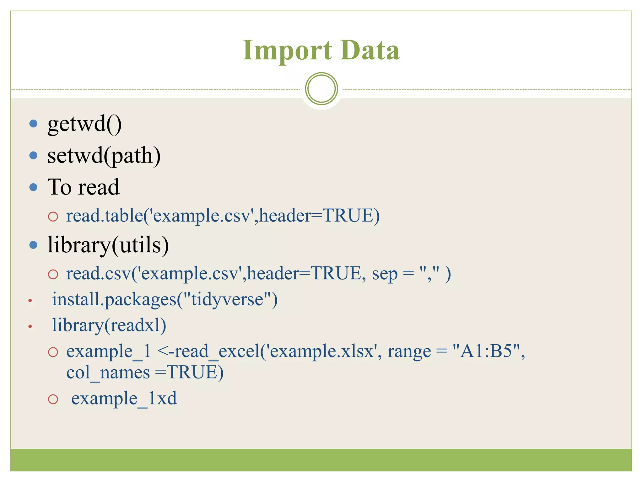
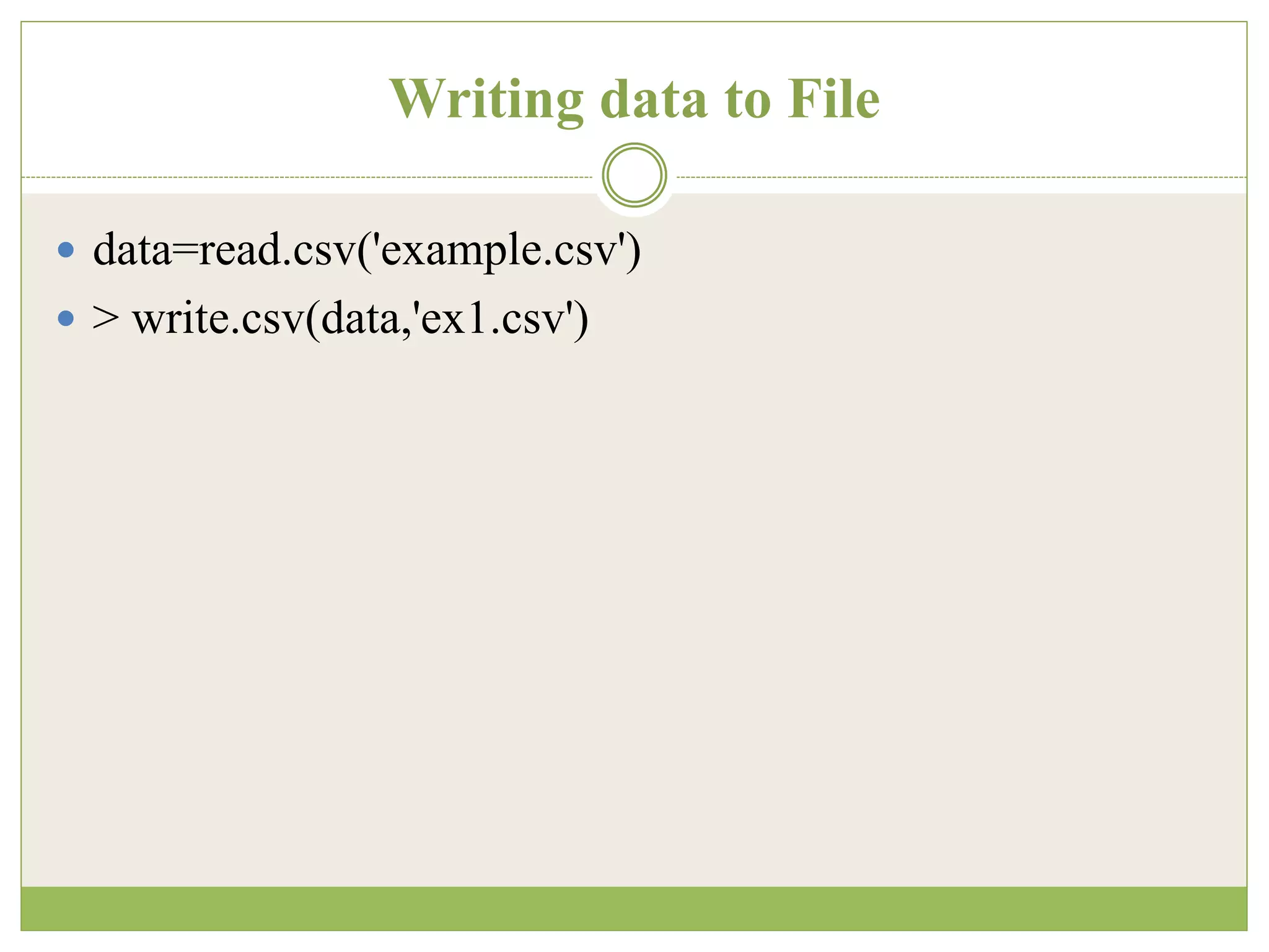
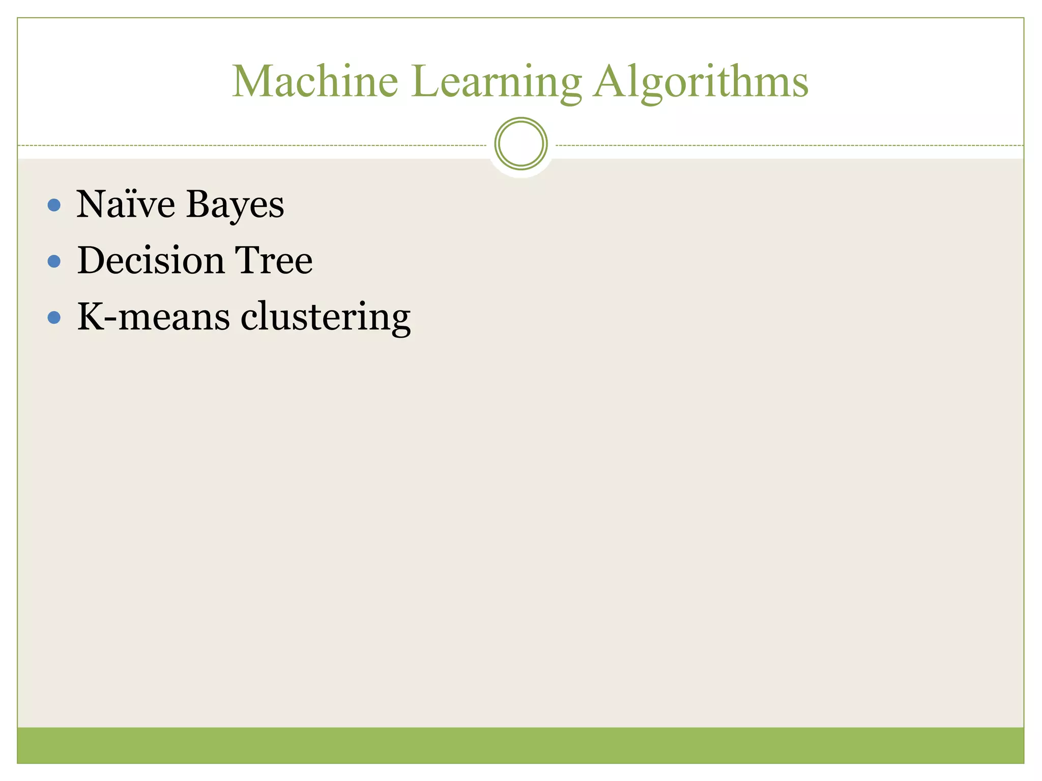
This document provides an overview of R programming. It discusses that R was developed in 1993 and is made up of libraries for data science. It covers basic R data types like vectors, matrices, data frames, and lists. It also describes how to import and export data from files in R and introduces several machine learning algorithms like Naive Bayes, decision trees, and k-means clustering.

1. H T T P S : / / W W W . G U R U 9 9 . C O M / R -
T U T O R I A L . H T M L
R Programming

2. Outline
 Introduction
 Data Types
 Import data to R/Export
 Machine Learning Algorithms

3. Introduction
 R is developed by Ross Ihaka and Robert Gentleman
in 1993.
 R is a clear and accessible programming tool.
 R is made up of a collection of libraries designed
specifically for data science.
 Investigate the data and analyze them.
 R provides a wide array of tools to capture the right
model for your data.

4. Introduction
 Uses
 Statistical inference
 Data analysis
 Machine learning algorithm

5. Data Types
 Basic Data types
 Scalars
 Vectors (numerical, character, logical)
 Matrices
 Data frames
 Lists

6. Basics types
 Numeric ( 3.5)
 Integers (5)
 Logical (True / False)
 Characters ( value inside “ ” or ‘ ’)

7. Declaration
# Declare variables of different types
# Numeric
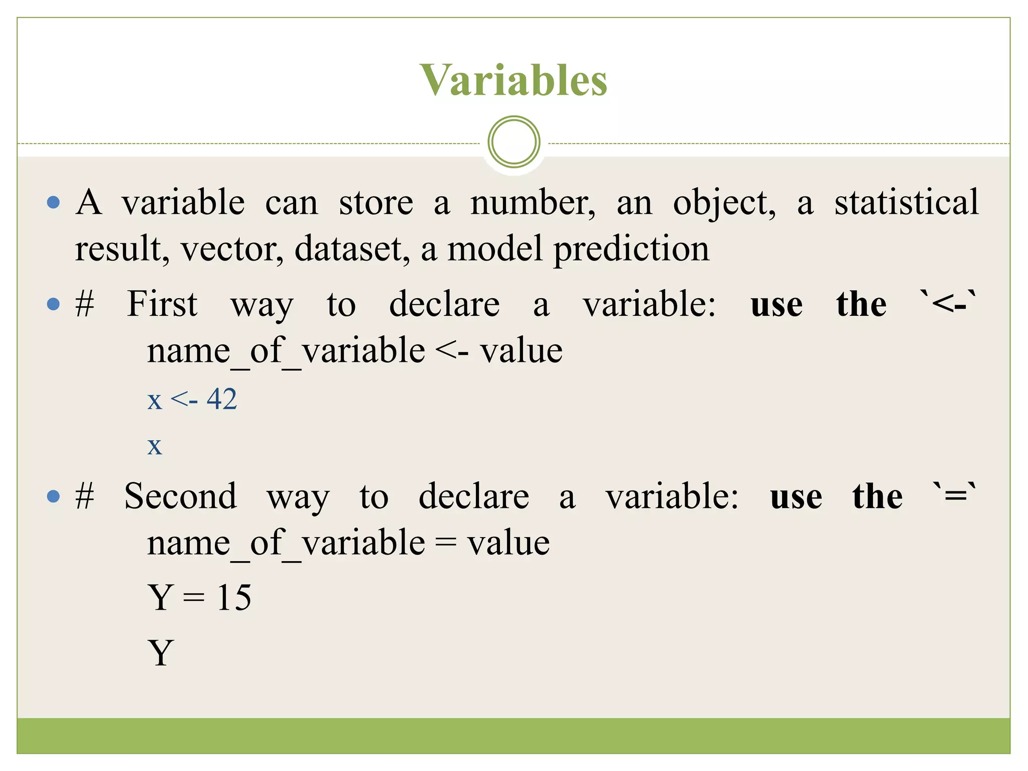
x <- 28
class(x)
Output:
## [1] "numeric“
# String
y <- "R Programming"
class(y)
Output:
## [1] "character“
# Boolean
z <- TRUE
class(z)
Output:
## [1] "logical"

8. Variables
 A variable can store a number, an object, a statistical
result, vector, dataset, a model prediction
 # First way to declare a variable: use the `<-`
name_of_variable <- value
x <- 42
x
 # Second way to declare a variable: use the `=`
name_of_variable = value
Y = 15
Y

9. Vectors
 A vector is a one-dimensional array.
# Numerical
vec_num <- c(1, 5, 10)
vec_num
# Character
vec_chr <- c("a", "b", "c")
vec_chr

10. Arithmetic calculations on vectors
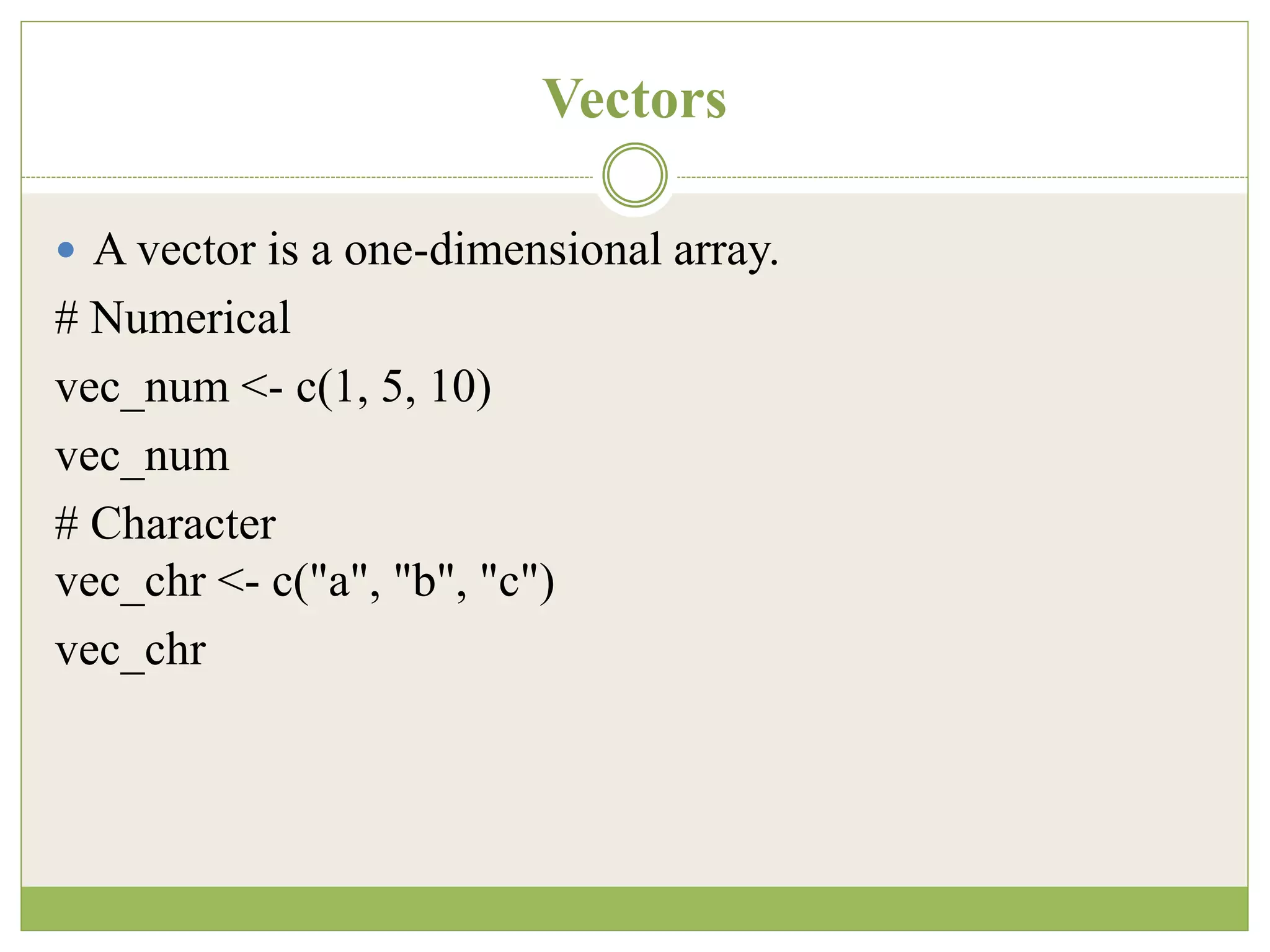
# Create the vectors
vect_1 <- c(1, 3, 5)
vect_2 <- c(2, 4, 6)
# Take the sum of A_vector and B_vector sum_vect <-
vect_1 + vect_2
# Print out total_vector
sum_vect
Output:
[1] 3 7 11

11. Slice operation
# Slice the first five rows of the vector
slice_vector <- c(1,2,3,4,5,6,7,8,9,10) slice_vector[1:5]
Output:
## [1] 1 2 3 4 5
# Faster way to create adjacent values
c(1:10)

12. Matrix
 2-dimensional array
 Create a Matrix in R
 matrix(data, nrow, ncol, byrow = FALSE)
data: The collection of elements that R will arrange into the rows and columns of
the matrix
nrow: Number of rows
ncol: Number of columns
byrow: The rows are filled from the left to the right. We use `byrow = FALSE`
(default values), if we want the matrix to be filled by the columns i.e. the values are
filled top to bottom.
 # Print dimension of the matrix with dim()
 dim(matrix_a)
 matrix_a <-matrix(1:10, byrow = TRUE, nrow = 5)
 matrix_b <-matrix(1:10, byrow = FALSE, nrow = 5)

13. Add a Column to a Matrix
 matrix_a <-matrix(1:10, byrow = TRUE, nrow = 5)
 matrix_a
 matrix_b <-matrix(11:20, byrow = FALSE, ncol = 2)
 matrix_b
 # concatenate matrix_b to the matrix_a
 matrix_a1 <- cbind(matrix_a, matrix_b)
 matrix_a1

14. Adding Row to a Matrix
matrix_c <-matrix(1:12, byrow = FALSE, ncol = 3)
matrix_c
# Create a vector of 3 columns
add_row <- c(1:3)
add_row
# Append to the matrix
matrix_c1 <- rbind(matrix_c, add_row)
matrix_c1
# Check the dimension
dim(matrix_c1)

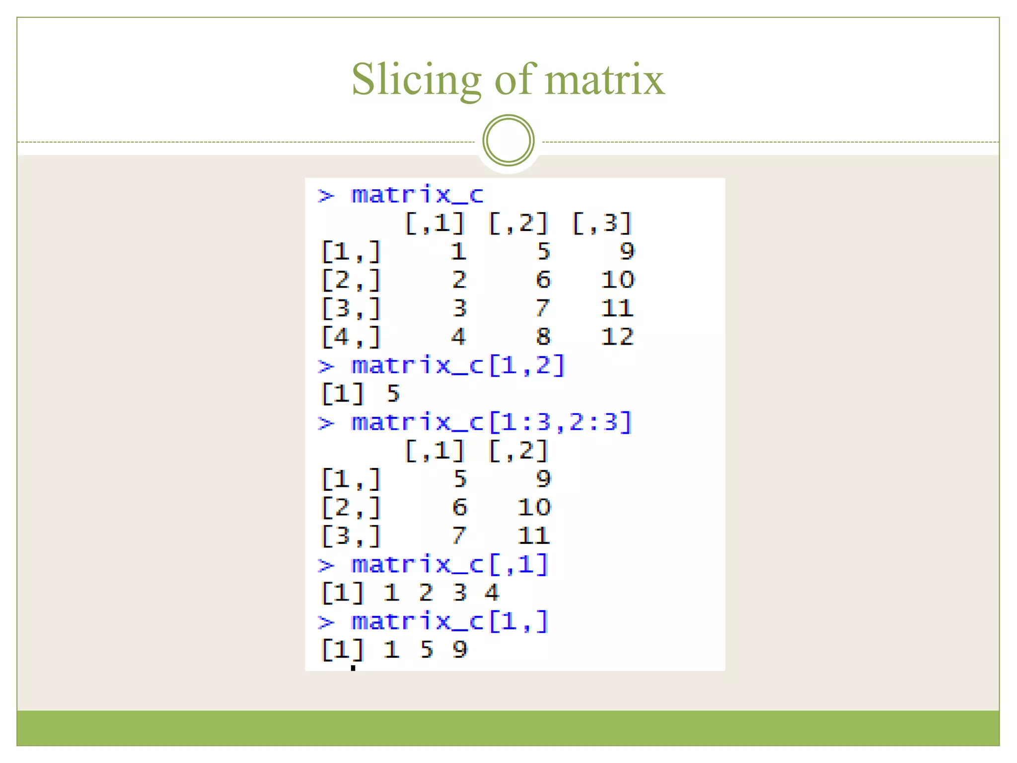
15. Slice a Matrix
 matrix_c[1,2] selects the element at the first row and
second column.
 matrix_c[1:3,2:3] results in a matrix with the data on
the rows 1, 2, 3 and columns 2, 3,
 matrix_c[,1] selects all elements of the first column.
 matrix_c[1,] selects all elements of the first row.

16. Slicing of matrix

17. Data Frame
 a list of vectors which are of equal length.
 A matrix contains only one type of data, while a data
frame accepts different data types (numeric, character,
factor, etc.).
 Create a Data Frame
 data.frame(df, stringsAsFactors = TRUE)
df: It can be a matrix to convert as a data frame or a collection of
variables to join
stringsAsFactors: Convert string to factor by default

18. Creating Data set
# Create a, b, c, d variables
a <- c(10,20,30,40)
b <- c('book', 'pen', 'text', 'pencil')
c <- c(TRUE,FALSE,TRUE,FALSE)
d <- c(2.5, 8, 10, 7)
# Join the variables to create a data frame
df <- data.frame(a,b,c,d)
df
Output
## a b c d
## 1 10 book TRUE 2.5
## 2 20 pen TRUE 8.0
## 3 30 text TRUE 10.0
## 4 40 pencil FALSE 7.0

19. Name the data frame and print structure
# Name the data frame
> names(df) <- c('ID', 'items', 'store', 'price')
> df
## ID items store price
## 1 10 book TRUE 2.5
## 2 20 pen FALSE 8.0
## 3 30 text TRUE 10.0
## 4 40 pencil FALSE 7.0
# Print the structure
str(df)

20. Slicing of Data frames

21. Select a Column of a Data Frame, Subset
 # Select the column ID
>df$ID
 Subset a Data Frame
 subset(x, condition)
 arguments: -
x: data frame used to perform the subset - condition: define
the conditional statement
# Select price above 5
subset(df, subset = price > 5)

22. List
 list is a great tool to store many kinds of object in the
order expected.
 A list can include matrices, vectors data and frames.
 list(element_1, ...)
 -element_1: store any type of R object

23. Creation of List
# Vector with numeric from 1 up to 5
vect <- 1:5
# A 2x 5 matrix
mat <- matrix(1:9, ncol = 5)
dim(mat)
# Construct list with these vec and mat
my_list <- list(vect, mat)
my_list
# Print second element of the list
my_list[[2]]

24. Import Data
 getwd()
 setwd(path)
 To read
 read.table('example.csv',header=TRUE)
 library(utils)
 read.csv('example.csv',header=TRUE, sep = "," )
• install.packages("tidyverse")
• library(readxl)
 example_1 <-read_excel('example.xlsx', range = "A1:B5",
col_names =TRUE)
 example_1xd

25. Writing data to File
 data=read.csv('example.csv')
 > write.csv(data,'ex1.csv')

26. Machine Learning Algorithms
 Naïve Bayes
 Decision Tree
 K-means clustering

27. THANK YOU