Download as PDF, PPTX


![Bayesian Models in R 10/3/14, 13:37
Condi6onal*Probability
A priori
Goal: find the items with strong relationships
First, load the data:
·
·
library(arules)
data = read.csv(data/BASKETS1n)
names(data)
[1] cardid value pmethod sex homeown income
[7] age fruitveg freshmeat dairy cannedveg cannedmeat
[13] frozenmeal beer wine softdrink fish confectionery
20/53
http://docs.supstat.com/BayesianModelEN/#1 Page 20 of 53](https://image.slidesharecdn.com/bayesianmodelsinr-141003123753-phpapp01/85/Bayesian-models-in-r-20-320.jpg)
![Bayesian Models in R 10/3/14, 13:37
Condi6onal*Probability
A priori
basket = data[, 8:18]
names(basket)[which(basket[1, ] == T)]
[1] freshmeat dairy confectionery
tbs2 = apply(basket, 1, function(x) names(basket)[which(x==T)])
len = sapply(tbs2, length)
require(arules)
trans.code = rep(1:1000, len)
trans.items = unname(unlist(tbs2))
trans.code.ind = match(trans.code, unique(trans.code))
trans.items.ind = match(trans.items, unique(trans.items))
21/53
http://docs.supstat.com/BayesianModelEN/#1 Page 21 of 53](https://image.slidesharecdn.com/bayesianmodelsinr-141003123753-phpapp01/85/Bayesian-models-in-r-21-320.jpg)

![Bayesian Models in R 10/3/14, 13:37
Condi6onal*Probability
A priori
parameter specification:
confidence minval smax arem aval originalSupport support minlen maxlen target ext
0.05 0.1 1 none FALSE TRUE 0.05 2 3 rules FALSE
algorithmic control:
filter tree heap memopt load sort verbose
0.1 TRUE TRUE FALSE TRUE 2 TRUE
apriori - find association rules with the apriori algorithm
version 4.21 (2004.05.09) (c) 1996-2004 Christian Borgelt
set item appearances ...[0 item(s)] done [0.00s].
set transactions ...[11 item(s), 940 transaction(s)] done [0.00s].
sorting and recoding items ... [11 item(s)] done [0.00s].
creating transaction tree ... done [0.00s].
checking subsets of size 1 2 3 done [0.00s].
writing ... [108 rule(s)] done [0.00s]. 23/53
http://docs.supstat.com/BayesianModelEN/#1 Page 23 of 53](https://image.slidesharecdn.com/bayesianmodelsinr-141003123753-phpapp01/85/Bayesian-models-in-r-23-320.jpg)
![Bayesian Models in R 10/3/14, 13:37
Condi6onal*Probability
· At last, we have the items with the strongest relationship in one basket
#let's see these rules:
lhs.generic = unique(trans.items)[trans.res@lhs@data@i+1]
rhs.generic = unique(trans.items)[trans.res@rhs@data@i+1]
cbind(lhs.generic, rhs.generic)[1:10, ]
lhs.generic rhs.generic
[1,] dairy confectionery
[2,] confectionery dairy
[3,] dairy fish
[4,] fish dairy
[5,] dairy fruitveg
[6,] fruitveg dairy
[7,] dairy frozenmeal
[8,] frozenmeal dairy
[9,] freshmeat confectionery
[10,] confectionery freshmeat
24/53
http://docs.supstat.com/BayesianModelEN/#1 Page 24 of 53](https://image.slidesharecdn.com/bayesianmodelsinr-141003123753-phpapp01/85/Bayesian-models-in-r-24-320.jpg)

![Bayesian Models in R 10/3/14, 13:37
Naive*Bayes
data(iris)
m = naiveBayes(Species ~ ., data=iris)
## alternatively:
m = naiveBayes(iris[, -5], iris[, 5])
26/53
http://docs.supstat.com/BayesianModelEN/#1 Page 26 of 53](https://image.slidesharecdn.com/bayesianmodelsinr-141003123753-phpapp01/85/Bayesian-models-in-r-26-320.jpg)
![Bayesian Models in R 10/3/14, 13:37
Naive*Bayes
Model:
m
Naive Bayes Classifier for Discrete Predictors
Call:
naiveBayes.default(x = iris[, -5], y = iris[, 5])
A-priori probabilities:
iris[, 5]
setosa versicolor virginica
0.33333 0.33333 0.33333
Conditional probabilities:
Sepal.Length
iris[, 5] [,1] [,2]
setosa 5.006 0.35249 27/53
http://docs.supstat.com/BayesianModelEN/#1 Page 27 of 53](https://image.slidesharecdn.com/bayesianmodelsinr-141003123753-phpapp01/85/Bayesian-models-in-r-27-320.jpg)
![Bayesian Models in R 10/3/14, 13:37
Naive*Bayes
Predict:
table(predict(m, iris), iris[,5])
setosa versicolor virginica
setosa 50 0 0
versicolor 0 47 3
virginica 0 3 47
28/53
http://docs.supstat.com/BayesianModelEN/#1 Page 28 of 53](https://image.slidesharecdn.com/bayesianmodelsinr-141003123753-phpapp01/85/Bayesian-models-in-r-28-320.jpg)


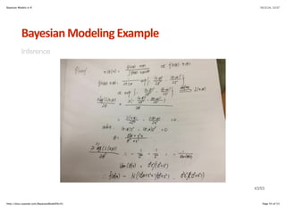
![Bayesian Models in R 10/3/14, 13:37
Bayesian*Models
Bayesian thinking
· The frequency perspective: The mean μ is a constant
colMeans(iris[, 1:3])
Sepal.Length Sepal.Width Petal.Length
5.8433 3.0573 3.7580
38/53
http://docs.supstat.com/BayesianModelEN/#1 Page 38 of 53](https://image.slidesharecdn.com/bayesianmodelsinr-141003123753-phpapp01/85/Bayesian-models-in-r-38-320.jpg)


![Bayesian Models in R 10/3/14, 13:37
Bayesian*Modeling*Example
Calculating the posterior distribution
According to the theorem, we know the mean and the variance of θ for a normal distribution.
postDis = function(miu=2, tau=4, n=100) {
x = rnorm(n,3,5)
a = list(0)
a[[1]] = (var(x)*miu+tau^2*mean(x))/(var(x)+tau^2)
a[[2]] = var(x)*tau^2/(var(x)+tau^2)
a
}
postDis(3, 5, 1000)
[[1]]
[1] 2.9284
[[2]]
[1] 12.254
44/53
http://docs.supstat.com/BayesianModelEN/#1 Page 44 of 53](https://image.slidesharecdn.com/bayesianmodelsinr-141003123753-phpapp01/85/Bayesian-models-in-r-44-320.jpg)


The document provides an overview of Bayesian models in R, including an introduction to Bayes' theorem and its applications in statistical modeling. It covers topics such as conditional probability, distribution estimation, and techniques for building Bayesian models, including the computation of posterior distributions. Practical examples are presented, including the use of Naive Bayes for classification and the application of the apriori algorithm for association rule mining.