bayesian regression is a probablistic method using in machine learning algorithms

1. Bayesian Linear Regression

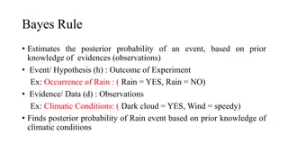
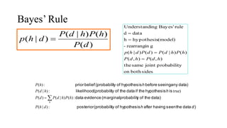
2. Bayes Rule
• Estimates the posterior probability of an event, based on prior
knowledge of evidences (observations)
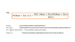
• Event/ Hypothesis (h) : Outcome of Experiment
Ex: Occurrence of Rain : ( Rain = YES, Rain = NO)
• Evidence/ Data (d) : Observations
Ex: Climatic Conditions: ( Dark cloud = YES, Wind = speedy)
• Finds posterior probability of Rain event based on prior knowledge of
climatic conditions

3. Bayes’ Rule
)
(
)
(
)
|
(
)
|
(
d
P
h
P
h
d
P
d
h
p 
)
data
the
seen
having
after
hypothesis
of
ty
(probabili
posterior
data)
the
of
y
probabilit
(marginal
evidence
data
is
hypothesis
the
if
data
the
of
ty
(probabili
likelihood
data)
any
seeing
before
hypothesis
of
ty
(probabili
belief
prior
d
h
h
h
:
)
|
(
:
)
(
)
|
(
)
(
true)
:
)
|
(
:
)
(
d
h
P
h
P
h
d
P
d
P
h
d
P
h
P
h


sides
both
on
y
probabilit
joint
same
the
)
,
(
)
,
(
)
(
)
|
(
)
(
)
|
(
g
rearrangin
-
(model)
hypothesis
h
data
d
rule
Bayes'
ing
Understand
h
d
P
h
d
P
h
P
h
d
P
d
P
d
h
p





4. • Ex:
)
(
)
(
)
|
(
)
|
(
C
P
Yes
Rain
P
Yes
Rain
C
P
C
Yes
Rain
P




)
conditions
climatic
the
on
based
Rain
getting
of
ty
(probabili
Posterior
evidence?
getting
of
y
probabilit
the
is
what
(Rain)
outcome
past
the
(Given
likelihood
)
Rain
the
getrting
of
ty
(probabili
belief
prior
:
)
|
(
evidence
the
getting
of
y
probabilit
Prior
:
)
(
)
|
(
)
(
)
:
)
|
(
:
)
(
C
Rain
P
Rain
P
Rain
C
P
C
P
Rain
C
P
Rain
P
h



5. Example of Bayes Theorem
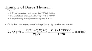
• Given:
• A doctor knows that covid causes fever 50% of the time
• Prior probability of any patient having covid is 1/50,000
• Prior probability of any patient having fever is 1/20
• If a patient has fever, what’s the probability he/she has covid?
0002
.
0
20
/
1
50000
/
1
5
.
0
)
(
)
(
)
|
(
)
|
( 



S
P
M
P
M
S
P
S
M
P

6. Linear Regression
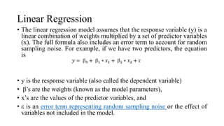
• The linear regression model assumes that the response variable (y) is a
linear combination of weights multiplied by a set of predictor variables
(x). The full formula also includes an error term to account for random
sampling noise. For example, if we have two predictors, the equation
is
• y is the response variable (also called the dependent variable)
• β’s are the weights (known as the model parameters),
• x’s are the values of the predictor variables, and
• ε is an error term representing random sampling noise or the effect of
variables not included in the model.

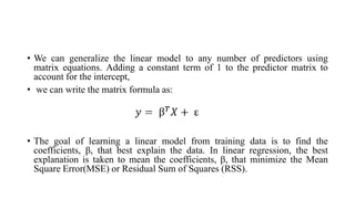
7. • We can generalize the linear model to any number of predictors using
matrix equations. Adding a constant term of 1 to the predictor matrix to
account for the intercept,
• we can write the matrix formula as:
• The goal of learning a linear model from training data is to find the
coefficients, β, that best explain the data. In linear regression, the best
explanation is taken to mean the coefficients, β, that minimize the Mean
Square Error(MSE) or Residual Sum of Squares (RSS).

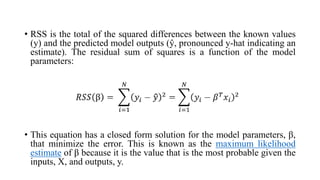
8. • RSS is the total of the squared differences between the known values
(y) and the predicted model outputs (ŷ, pronounced y-hat indicating an
estimate). The residual sum of squares is a function of the model
parameters:
• This equation has a closed form solution for the model parameters, β,
that minimize the error. This is known as the maximum likelihood
estimate of β because it is the value that is the most probable given the
inputs, X, and outputs, y.

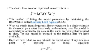
9. • The closed form solution expressed in matrix form is:
• This method of fitting the model parameters by minimizing the
RSS/MSE is called Ordinary Least Squares (OLS).
• What we obtain from frequentist linear regression is a single estimate
for the model parameters based only on the training data. Our model is
completely informed by the data: in this view, everything that we need
to know for our model is encoded in the training data we have
available.
• Once we have β-hat, we can estimate the output value of any new data
point by applying our model equation:

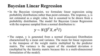
10. Bayesian Linear Regression
• In the Bayesian viewpoint, we formulate linear regression using
probability distributions rather than point estimates. The response, y, is
not estimated as a single value, but is assumed to be drawn from a
probability distribution. The model for Bayesian Linear Regression
with the response sampled from a normal distribution is:
• The output, y is generated from a normal (Gaussian) Distribution
characterized by a mean and variance. The mean for linear regression
is the transpose of the weight matrix multiplied by the predictor
matrix. The variance is the square of the standard deviation σ
(multiplied by the Identity matrix because this is a multi-dimensional
formulation of the model).

11. • The aim of Bayesian Linear Regression is not to find the single “best”
value of the model parameters, but rather to determine the posterior
distribution for the model parameters.
• Not only is the response generated from a probability distribution, but
the model parameters are assumed to come from a distribution as well.

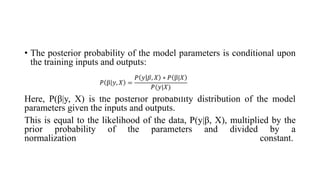
12. • The posterior probability of the model parameters is conditional upon
the training inputs and outputs:
Here, P(β|y, X) is the posterior probability distribution of the model
parameters given the inputs and outputs.
This is equal to the likelihood of the data, P(y|β, X), multiplied by the
prior probability of the parameters and divided by a
normalization constant.

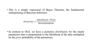
13. • This is a simple expression of Bayes Theorem, the fundamental
underpinning of Bayesian Inference:
• In contrast to OLS, we have a posterior distribution for the model
parameters that is proportional to the likelihood of the data multiplied
by the prior probability of the parameters

14. Primary benefits of Bayesian Linear
Regression.
• Priors: If we have domain knowledge, or a guess for what the model
parameters should be, we can include them in our model, unlike in the
frequentist approach which assumes everything there is to know about
the parameters comes from the data. If we don’t have any estimates
ahead of time, we can use non-informative priors for the parameters
such as a normal distribution.
• Posterior: The result of performing Bayesian Linear Regression is a
distribution of possible model parameters based on the data and the
prior. This allows us to quantify our uncertainty about the model: if we
have fewer data points, the posterior distribution will be more spread
out.