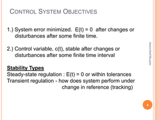
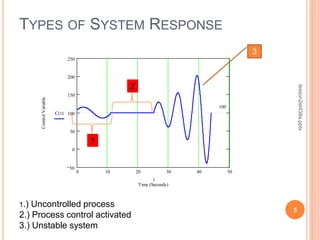
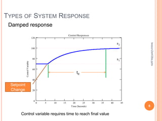
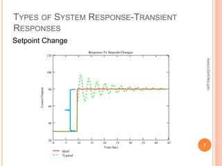
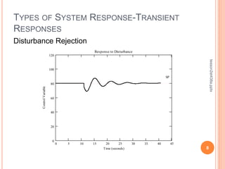
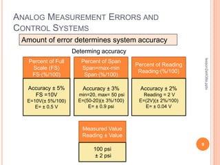
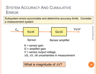
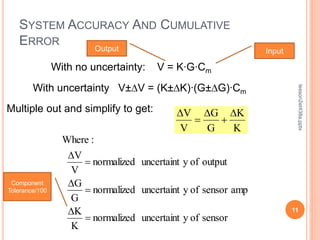
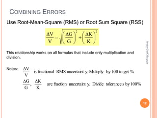
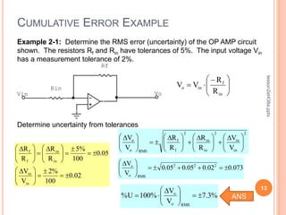
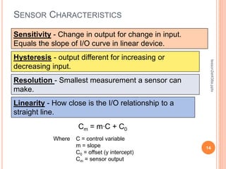
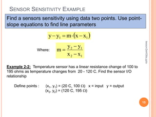
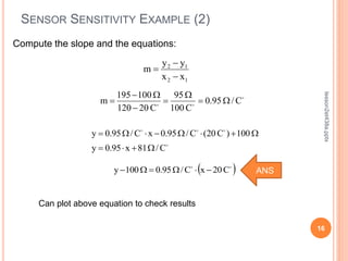
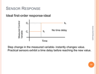
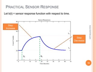
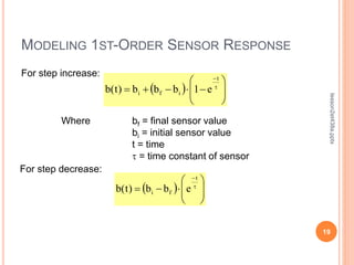
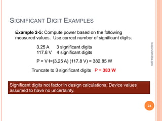
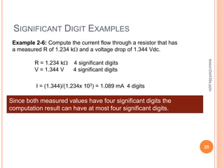
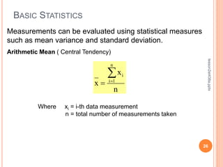
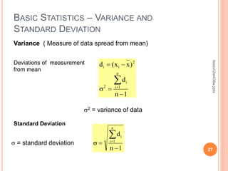
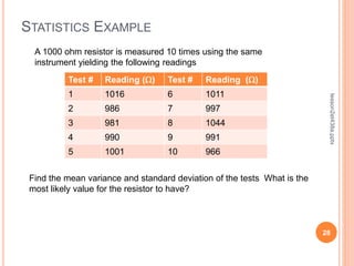
LESSON 2: PERFORMANCE OF
CONTROL SYSTEMS
ET 438a
Automatic Control Systems Technology
1
lesson2et438a.pptx
lesson2et438a.pptx
2
LEARNING OBJECTIVES
After this presentation you will be able to:
 Explain what constitutes good control system
performance.
 Identify controlled, uncontrolled, and unstable
control system response.
 Analyze measurement error in measurement
sensors.
 Determine sensor response.
 Apply significant digits and basic statistics to
analyze measurements.
CONTROL SYSTEM PERFORMANCE
3
lesson2et438a.pptx
E(t) = R - C(t)
Where E(t) = error as a function of time
R = setpoint (reference) value
C(t) = control variable as a function of time
System control variable changes over time so error
changes with time.
Determine performance criteria for adequate control
system performance. System should maintain desired
output as closely as possible when subjected to
disturbances and other changes
CONTROL SYSTEM OBJECTIVES
4
lesson2et438a.pptx
1.) System error minimized. E(t) = 0 after changes or
disturbances after some finite time.
2.) Control variable, c(t), stable after changes or
disturbances after some finite time interval
Stability Types
Steady-state regulation : E(t) = 0 or within tolerances
Transient regulation - how does system perform under
change in reference (tracking)
TYPES OF SYSTEM RESPONSE
5
lesson2et438a.pptx
0 10 20 30 40 50
50
0
50
100
150
200
250
Time (Seconds)
Control
Variable
100
C t
( )
t
1.) Uncontrolled process
2.) Process control activated
3.) Unstable system
1
3
2
TYPES OF SYSTEM RESPONSE
6
lesson2et438a.pptx
Damped response
0 5 10 15 20 25 30 35 40 45
0
20
40
60
80
100
120
Control Responses
Time (Seconds)
Control
Variable
R1
R2
Setpoint
Change
td
Control variable requires time to reach final value
TYPES OF SYSTEM RESPONSE-TRANSIENT
RESPONSES
7
lesson2et438a.pptx
0 5 10 15 20 25 30 35 40 45
20
40
60
80
100
120
Ideal
Typical
Response To Setpoint Changes
Time (Sec)
Control
Outputs
Setpoint Change
TYPES OF SYSTEM RESPONSE-TRANSIENT
RESPONSES
8
lesson2et438a.pptx
Disturbance Rejection
0 5 10 15 20 25 30 35 40 45
0
20
40
60
80
100
120
Response to Disturbance
Time (seconds)
Control
Variable
SP
ANALOG MEASUREMENT ERRORS AND
CONTROL SYSTEMS
9
lesson2et438a.pptx
Amount of error determines system accuracy
Determing accuracy
Measured Value
Reading ± Value
100 psi
± 2 psi
Percent of Full
Scale (FS)
FS∙(%/100)
Accuracy ± 5%
FS =10V
E=10V(± 5%/100)
E= ± 0.5 V
Percent of Span
Span=max-min
Span∙(%/100)
Accuracy ± 3%
min=20, max= 50 psi
E=(50-20)(± 3%/100)
E= ± 0.9 psi
Percent of Reading
Reading∙(%/100)
Accuracy ± 2%
Reading = 2 V
E=(2V)(± 2%/100)
E= ± 0.04 V
SYSTEM ACCURACY AND CUMULATIVE
ERROR
10
lesson2et438a.pptx
Sensor Sensor amplifier
Subsystem errors accumulate and determine accuracy limits. Consider
a measurement system
K±DK
Cm
G±DG
V±DV
K = sensor gain
G = amplifier gain
V = sensor output voltage,
DG, DV, DK uncertainties in measurement
What is magnitude of DV?
SYSTEM ACCURACY AND CUMULATIVE
ERROR
11
lesson2et438a.pptx
With no uncertainty: V = K∙G∙Cm
With uncertainty V±DV = (K±DK)∙(G±DG)∙Cm
Multiple out and simplify to get:
Input
Output
K
K
G
G
V
V D

D

D
sensor
of
y
uncertaint
normalized
K
K
amp
sensor
of
y
uncertaint
normalized
G
G
output
of
y
uncertaint
normalized
V
V
:
Where

D

D

D
Component
Tolerance/100
COMBINING ERRORS
12
lesson2et438a.pptx
Use Root-Mean-Square (RMS) or Root Sum Square (RSS)
2
2
K
K
G
G
V
V





 D






 D

D
This relationship works on all formulas that include only multiplication and
division.
Notes:
100%
by
s
tolerance
Divide
y.
uncertaint
fraction
are
K
K
,
G
G
%
get
to
100
by
Multiply
.
y
uncertaint
RMS
fractional
is
V
V
D
D
D
CUMULATIVE ERROR EXAMPLE
13
lesson2et438a.pptx
Example 2-1: Determine the RMS error (uncertainty) of the OP AMP circuit
shown. The resistors Rf and Rin have tolerances of 5%. The input voltage Vin
has a measurement tolerance of 2%.
Vo
Rin
Rf
Vin







 


in
f
in
o
R
R
V
V
Determine uncertainty from tolerances
02
.
0
100
%
2
V
V
05
.
0
100
%
5
R
R
R
R
in
in
in
in
f
f











 D











 D








 D
2
in
in
2
in
in
2
f
f
RMS
o
o
V
V
R
R
R
R
V
V







 D








 D








 D









 D
073
.
0
02
.
0
05
.
0
05
.
0
V
V 2
2
2
RMS
o
o













 D
%
3
.
7
V
V
%
100
U
%
RMS
o
o









 D

 ANS
SENSOR CHARACTERISTICS
14
lesson2et438a.pptx
Sensitivity - Change in output for change in input.
Equals the slope of I/O curve in linear device.
Hysteresis - output different for increasing or
decreasing input.
Resolution - Smallest measurement a sensor can
make.
Linearity - How close is the I/O relationship to a
straight line.
Cm = m∙C + C0
Where C = control variable
m = slope
C0 = offset (y intercept)
Cm = sensor output
SENSOR SENSITIVITY EXAMPLE
15
lesson2et438a.pptx
Find a sensors sensitivity using data two points. Use point-
slope equations to find line parameters
 
1
1 x
x
m
y
y 



1
2
1
2
x
x
y
y
m



Where:
Example 2-2: Temperature sensor has a linear resistance change of 100 to
195 ohms as temperature changes from 20 - 120 C. Find the sensor I/O
relationship
Define points : (x1, y1) = (20 C, 100 W) x = input y = output
(x2, y2) = (120 C, 195 W)
lesson2et438a.pptx
16
SENSOR SENSITIVITY EXAMPLE (2)
1
2
1
2
x
x
y
y
m






C
/
95
.
0
C
100
95
C
20
120
100
195
m W

W


W


 


C
20
x
C
/
95
.
0
100
y 

W

W





C
/
81
x
95
.
0
y
100
)
C
20
(
C
/
95
.
0
x
C
/
95
.
0
y
W



W


W


W

Compute the slope and the equations:
Can plot above equation to check results
ANS
SENSOR RESPONSE
17
lesson2et438a.pptx
Ideal first-order response-ideal
bi
bf
Ci
Cf
No time delay
Time
Measured
Control
Variable
Step change in the measured variable- instantly changes value.
Practical sensors exhibit a time delay before reaching the new value.
PRACTICAL SENSOR RESPONSE
18
lesson2et438a.pptx
Let b(t) = sensor response function with respect to time.
0 5 10 15 20 25 30 35 40 45
0
20
40
60
80
Sensor Responses
Time (Seconds)
Control
Variable
bi
bf
Step
Decrease
Step
Increase
bi bf
MODELING 1ST-ORDER SENSOR RESPONSE
19
lesson2et438a.pptx
For step increase:
Where bf = final sensor value
bi = initial sensor value
t = time
t = time constant of sensor
  











 t
t
i
f
i e
1
b
b
b
)
t
(
b
For step decrease:
  









 t
t
f
i e
b
b
)
t
(
b
SENSOR RESPONSE EXAMPLE 1
20
lesson2et438a.pptx
Example 2-3: A control loop sensor detects a step increase
and has an initial voltage output of bi = 2.0 V Its final output is
bf = 4.0 V. It has a time constant of t = 0.0025 /s. Find the
time it takes to reach 90% of its final value.
EXAMPLE 2-3 CONTINUED (2)
21
lesson2et438a.pptx
Complete the calculations to find t
SENSOR RESPONSE EXAMPLE 2
22
lesson2et438a.pptx
Example 2-4: A sensor with a first order response characteristic
has initial output of 1.0 V. How long does it take to decrease to
0.2 V if the time constant of the sensor is 0.1/s.
SIGNIFICANT DIGITS IN INSTRUMENTATION
AND CONTROL
23
lesson2et438a.pptx
Significant Digits In Measurement
Readable output of instruments
Resolution of sensors and transducers
Calculations Using Measurements
Truncate calculator answers to match
significant digits of measurements and
readings,
SIGNIFICANT DIGIT EXAMPLES
24
lesson2et438a.pptx
Example 2-5: Compute power based on the following
measured values. Use correct number of significant digits.
Significant digits not factor in design calculations. Device values
assumed to have no uncertainty.
3.25 A 3 significant digits
117.8 V 4 significant digits
P = V∙I=(3.25 A)∙(117.8 V) = 382.85 W
Truncate to 3 significant digits P = 383 W
SIGNIFICANT DIGIT EXAMPLES
25
lesson2et438a.pptx
Example 2-6: Compute the current flow through a resistor that has
a measured R of 1.234 kW and a voltage drop of 1.344 Vdc.
R = 1.234 kW 4 significant digits
V = 1.344 V 4 significant digits
I = (1.344)/(1.234x 103) = 1.089 mA 4 digits
Since both measured values have four significant digits the
computation result can have at most four significant digits.
BASIC STATISTICS
26
lesson2et438a.pptx
Measurements can be evaluated using statistical measures
such as mean variance and standard deviation.
Arithmetic Mean ( Central Tendency)
n
x
x
n
1
i
i



Where xi = i-th data measurement
n = total number of measurements taken
BASIC STATISTICS – VARIANCE AND
STANDARD DEVIATION
27
lesson2et438a.pptx
1
n
d
)
x
x
(
d
n
1
i
i
2
2
i
i







Variance ( Measure of data spread from mean)
Deviations of measurement
from mean
2 = variance of data
Standard Deviation
 = standard deviation
1
n
d
n
1
i
i





STATISTICS EXAMPLE
28
lesson2et438a.pptx
A 1000 ohm resistor is measured 10 times using the same
instrument yielding the following readings
Test # Reading (W) Test # Reading (W)
1 1016 6 1011
2 986 7 997
3 981 8 1044
4 990 9 991
5 1001 10 966
Find the mean variance and standard deviation of the tests What is the
most likely value for the resistor to have?
STATISTICS EXAMPLE SOLUTION
29
lesson2et438a.pptx
Variance Calculations
END LESSON 2: PERFORMANCE OF
CONTROL SYSTEMS
ET 438a
Automatic Control Systems Technology
lesson2et438a.pptx
30

lesson2.ppsx

  • 1.
    LESSON 2: PERFORMANCEOF CONTROL SYSTEMS ET 438a Automatic Control Systems Technology 1 lesson2et438a.pptx
  • 2.
    lesson2et438a.pptx 2 LEARNING OBJECTIVES After thispresentation you will be able to:  Explain what constitutes good control system performance.  Identify controlled, uncontrolled, and unstable control system response.  Analyze measurement error in measurement sensors.  Determine sensor response.  Apply significant digits and basic statistics to analyze measurements.
  • 3.
    CONTROL SYSTEM PERFORMANCE 3 lesson2et438a.pptx E(t)= R - C(t) Where E(t) = error as a function of time R = setpoint (reference) value C(t) = control variable as a function of time System control variable changes over time so error changes with time. Determine performance criteria for adequate control system performance. System should maintain desired output as closely as possible when subjected to disturbances and other changes
  • 4.
    CONTROL SYSTEM OBJECTIVES 4 lesson2et438a.pptx 1.)System error minimized. E(t) = 0 after changes or disturbances after some finite time. 2.) Control variable, c(t), stable after changes or disturbances after some finite time interval Stability Types Steady-state regulation : E(t) = 0 or within tolerances Transient regulation - how does system perform under change in reference (tracking)
  • 5.
    TYPES OF SYSTEMRESPONSE 5 lesson2et438a.pptx 0 10 20 30 40 50 50 0 50 100 150 200 250 Time (Seconds) Control Variable 100 C t ( ) t 1.) Uncontrolled process 2.) Process control activated 3.) Unstable system 1 3 2
  • 6.
    TYPES OF SYSTEMRESPONSE 6 lesson2et438a.pptx Damped response 0 5 10 15 20 25 30 35 40 45 0 20 40 60 80 100 120 Control Responses Time (Seconds) Control Variable R1 R2 Setpoint Change td Control variable requires time to reach final value
  • 7.
    TYPES OF SYSTEMRESPONSE-TRANSIENT RESPONSES 7 lesson2et438a.pptx 0 5 10 15 20 25 30 35 40 45 20 40 60 80 100 120 Ideal Typical Response To Setpoint Changes Time (Sec) Control Outputs Setpoint Change
  • 8.
    TYPES OF SYSTEMRESPONSE-TRANSIENT RESPONSES 8 lesson2et438a.pptx Disturbance Rejection 0 5 10 15 20 25 30 35 40 45 0 20 40 60 80 100 120 Response to Disturbance Time (seconds) Control Variable SP
  • 9.
    ANALOG MEASUREMENT ERRORSAND CONTROL SYSTEMS 9 lesson2et438a.pptx Amount of error determines system accuracy Determing accuracy Measured Value Reading ± Value 100 psi ± 2 psi Percent of Full Scale (FS) FS∙(%/100) Accuracy ± 5% FS =10V E=10V(± 5%/100) E= ± 0.5 V Percent of Span Span=max-min Span∙(%/100) Accuracy ± 3% min=20, max= 50 psi E=(50-20)(± 3%/100) E= ± 0.9 psi Percent of Reading Reading∙(%/100) Accuracy ± 2% Reading = 2 V E=(2V)(± 2%/100) E= ± 0.04 V
  • 10.
    SYSTEM ACCURACY ANDCUMULATIVE ERROR 10 lesson2et438a.pptx Sensor Sensor amplifier Subsystem errors accumulate and determine accuracy limits. Consider a measurement system K±DK Cm G±DG V±DV K = sensor gain G = amplifier gain V = sensor output voltage, DG, DV, DK uncertainties in measurement What is magnitude of DV?
  • 11.
    SYSTEM ACCURACY ANDCUMULATIVE ERROR 11 lesson2et438a.pptx With no uncertainty: V = K∙G∙Cm With uncertainty V±DV = (K±DK)∙(G±DG)∙Cm Multiple out and simplify to get: Input Output K K G G V V D  D  D sensor of y uncertaint normalized K K amp sensor of y uncertaint normalized G G output of y uncertaint normalized V V : Where  D  D  D Component Tolerance/100
  • 12.
    COMBINING ERRORS 12 lesson2et438a.pptx Use Root-Mean-Square(RMS) or Root Sum Square (RSS) 2 2 K K G G V V       D        D  D This relationship works on all formulas that include only multiplication and division. Notes: 100% by s tolerance Divide y. uncertaint fraction are K K , G G % get to 100 by Multiply . y uncertaint RMS fractional is V V D D D
  • 13.
    CUMULATIVE ERROR EXAMPLE 13 lesson2et438a.pptx Example2-1: Determine the RMS error (uncertainty) of the OP AMP circuit shown. The resistors Rf and Rin have tolerances of 5%. The input voltage Vin has a measurement tolerance of 2%. Vo Rin Rf Vin            in f in o R R V V Determine uncertainty from tolerances 02 . 0 100 % 2 V V 05 . 0 100 % 5 R R R R in in in in f f             D             D          D 2 in in 2 in in 2 f f RMS o o V V R R R R V V         D          D          D           D 073 . 0 02 . 0 05 . 0 05 . 0 V V 2 2 2 RMS o o               D % 3 . 7 V V % 100 U % RMS o o           D   ANS
  • 14.
    SENSOR CHARACTERISTICS 14 lesson2et438a.pptx Sensitivity -Change in output for change in input. Equals the slope of I/O curve in linear device. Hysteresis - output different for increasing or decreasing input. Resolution - Smallest measurement a sensor can make. Linearity - How close is the I/O relationship to a straight line. Cm = m∙C + C0 Where C = control variable m = slope C0 = offset (y intercept) Cm = sensor output
  • 15.
    SENSOR SENSITIVITY EXAMPLE 15 lesson2et438a.pptx Finda sensors sensitivity using data two points. Use point- slope equations to find line parameters   1 1 x x m y y     1 2 1 2 x x y y m    Where: Example 2-2: Temperature sensor has a linear resistance change of 100 to 195 ohms as temperature changes from 20 - 120 C. Find the sensor I/O relationship Define points : (x1, y1) = (20 C, 100 W) x = input y = output (x2, y2) = (120 C, 195 W)
  • 16.
    lesson2et438a.pptx 16 SENSOR SENSITIVITY EXAMPLE(2) 1 2 1 2 x x y y m       C / 95 . 0 C 100 95 C 20 120 100 195 m W  W   W       C 20 x C / 95 . 0 100 y   W  W      C / 81 x 95 . 0 y 100 ) C 20 ( C / 95 . 0 x C / 95 . 0 y W    W   W   W  Compute the slope and the equations: Can plot above equation to check results ANS
  • 17.
    SENSOR RESPONSE 17 lesson2et438a.pptx Ideal first-orderresponse-ideal bi bf Ci Cf No time delay Time Measured Control Variable Step change in the measured variable- instantly changes value. Practical sensors exhibit a time delay before reaching the new value.
  • 18.
    PRACTICAL SENSOR RESPONSE 18 lesson2et438a.pptx Letb(t) = sensor response function with respect to time. 0 5 10 15 20 25 30 35 40 45 0 20 40 60 80 Sensor Responses Time (Seconds) Control Variable bi bf Step Decrease Step Increase bi bf
  • 19.
    MODELING 1ST-ORDER SENSORRESPONSE 19 lesson2et438a.pptx For step increase: Where bf = final sensor value bi = initial sensor value t = time t = time constant of sensor                t t i f i e 1 b b b ) t ( b For step decrease:              t t f i e b b ) t ( b
  • 20.
    SENSOR RESPONSE EXAMPLE1 20 lesson2et438a.pptx Example 2-3: A control loop sensor detects a step increase and has an initial voltage output of bi = 2.0 V Its final output is bf = 4.0 V. It has a time constant of t = 0.0025 /s. Find the time it takes to reach 90% of its final value.
  • 21.
    EXAMPLE 2-3 CONTINUED(2) 21 lesson2et438a.pptx Complete the calculations to find t
  • 22.
    SENSOR RESPONSE EXAMPLE2 22 lesson2et438a.pptx Example 2-4: A sensor with a first order response characteristic has initial output of 1.0 V. How long does it take to decrease to 0.2 V if the time constant of the sensor is 0.1/s.
  • 23.
    SIGNIFICANT DIGITS ININSTRUMENTATION AND CONTROL 23 lesson2et438a.pptx Significant Digits In Measurement Readable output of instruments Resolution of sensors and transducers Calculations Using Measurements Truncate calculator answers to match significant digits of measurements and readings,
  • 24.
    SIGNIFICANT DIGIT EXAMPLES 24 lesson2et438a.pptx Example2-5: Compute power based on the following measured values. Use correct number of significant digits. Significant digits not factor in design calculations. Device values assumed to have no uncertainty. 3.25 A 3 significant digits 117.8 V 4 significant digits P = V∙I=(3.25 A)∙(117.8 V) = 382.85 W Truncate to 3 significant digits P = 383 W
  • 25.
    SIGNIFICANT DIGIT EXAMPLES 25 lesson2et438a.pptx Example2-6: Compute the current flow through a resistor that has a measured R of 1.234 kW and a voltage drop of 1.344 Vdc. R = 1.234 kW 4 significant digits V = 1.344 V 4 significant digits I = (1.344)/(1.234x 103) = 1.089 mA 4 digits Since both measured values have four significant digits the computation result can have at most four significant digits.
  • 26.
    BASIC STATISTICS 26 lesson2et438a.pptx Measurements canbe evaluated using statistical measures such as mean variance and standard deviation. Arithmetic Mean ( Central Tendency) n x x n 1 i i    Where xi = i-th data measurement n = total number of measurements taken
  • 27.
    BASIC STATISTICS –VARIANCE AND STANDARD DEVIATION 27 lesson2et438a.pptx 1 n d ) x x ( d n 1 i i 2 2 i i        Variance ( Measure of data spread from mean) Deviations of measurement from mean 2 = variance of data Standard Deviation  = standard deviation 1 n d n 1 i i     
  • 28.
    STATISTICS EXAMPLE 28 lesson2et438a.pptx A 1000ohm resistor is measured 10 times using the same instrument yielding the following readings Test # Reading (W) Test # Reading (W) 1 1016 6 1011 2 986 7 997 3 981 8 1044 4 990 9 991 5 1001 10 966 Find the mean variance and standard deviation of the tests What is the most likely value for the resistor to have?
  • 29.
  • 30.
    END LESSON 2:PERFORMANCE OF CONTROL SYSTEMS ET 438a Automatic Control Systems Technology lesson2et438a.pptx 30