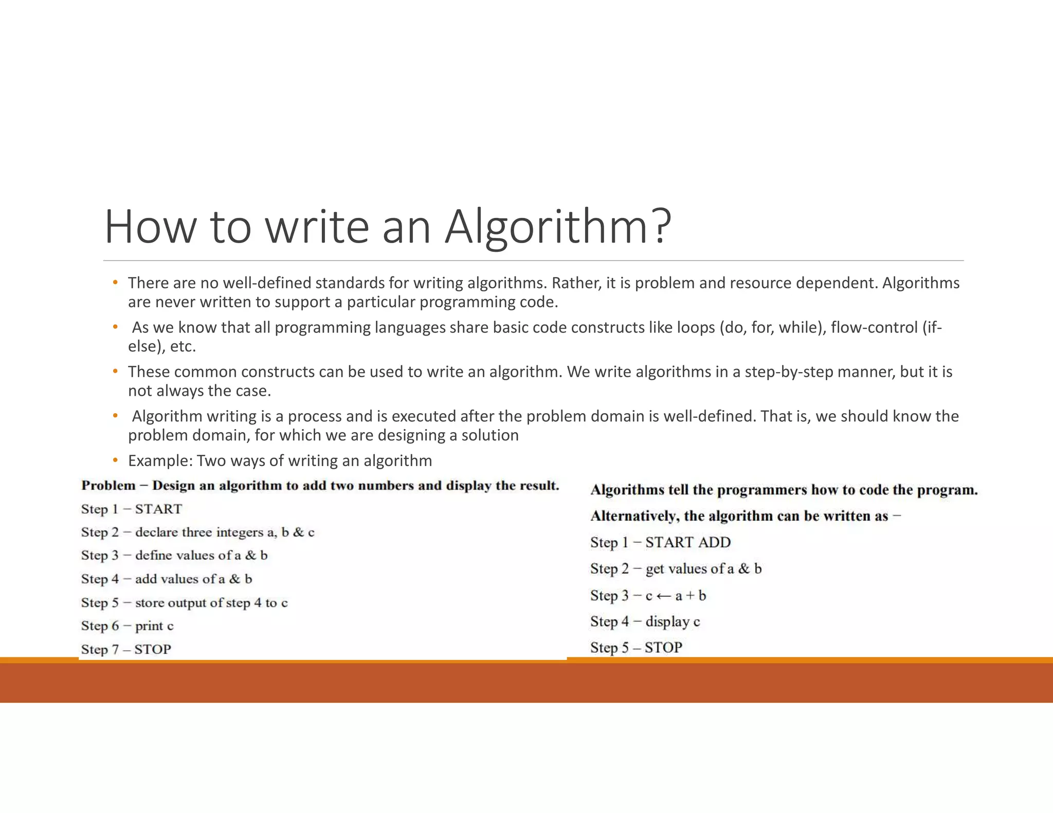
1. An algorithm is a step-by-step procedure to solve a problem using a finite number of well-defined instructions and inputs. An algorithm must be unambiguous, have a finite number of steps, and be feasible with available resources.
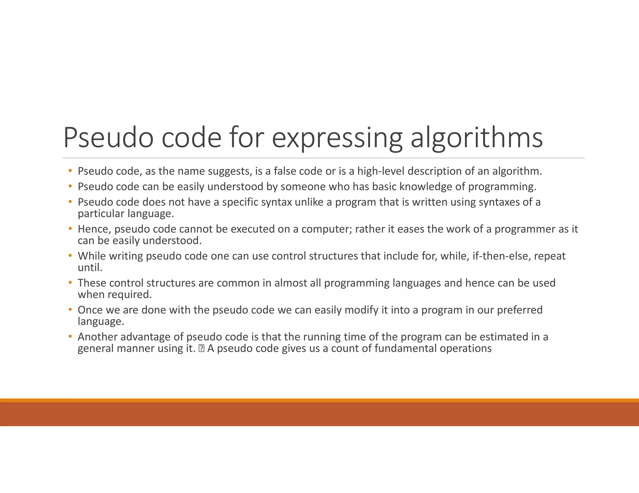
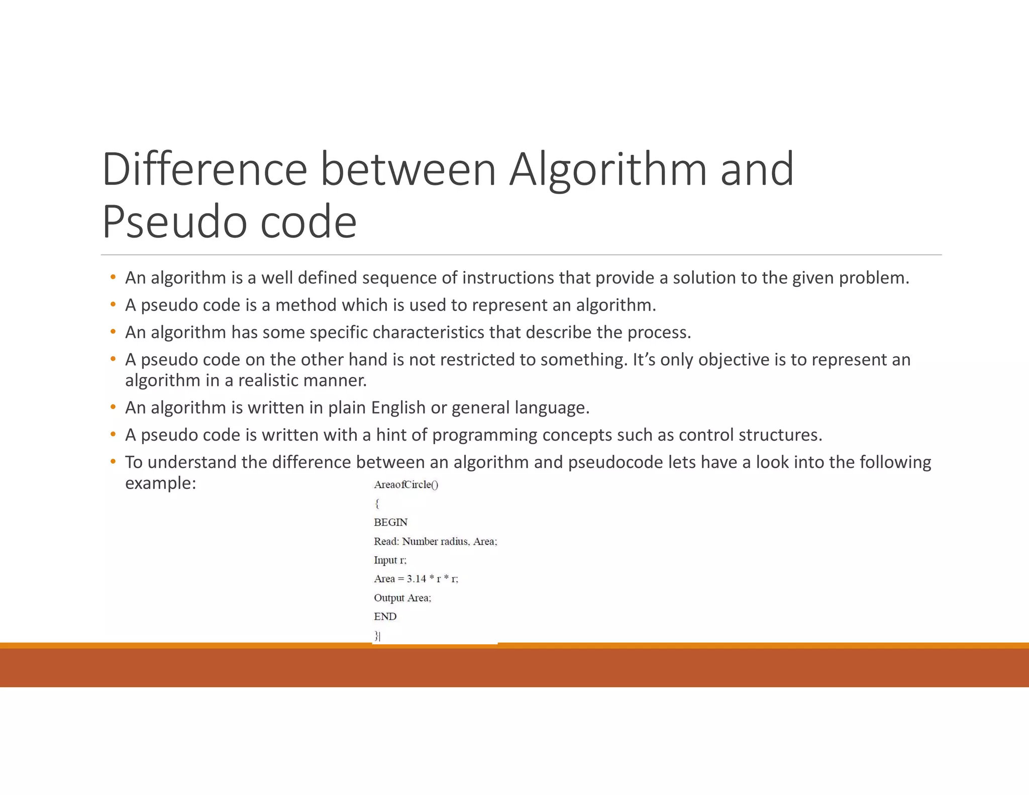
2. Pseudo code is used to represent algorithms without using a specific programming language syntax. It uses common programming constructs like loops and conditionals. Pseudo code improves readability and acts as a bridge between algorithms and programs.
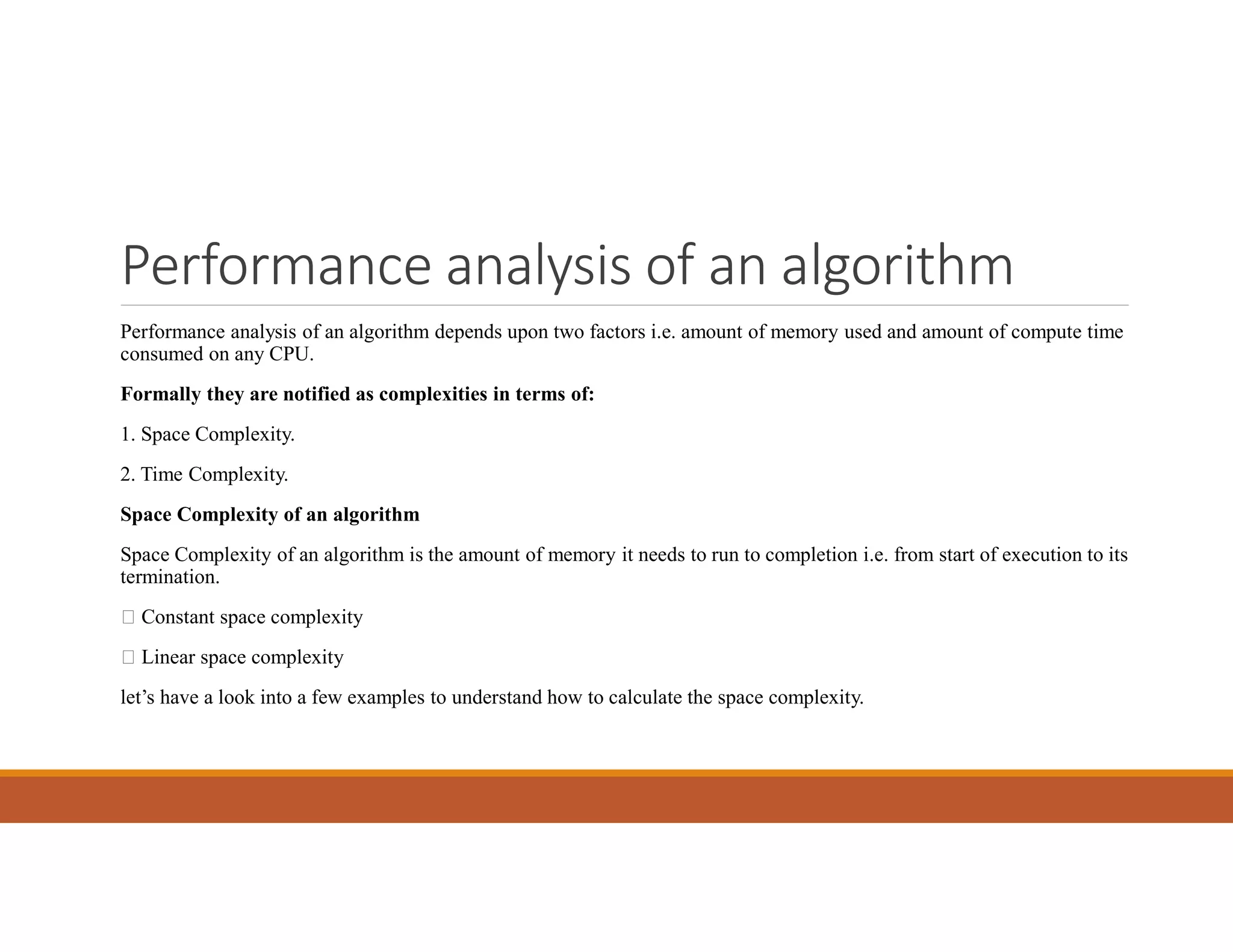
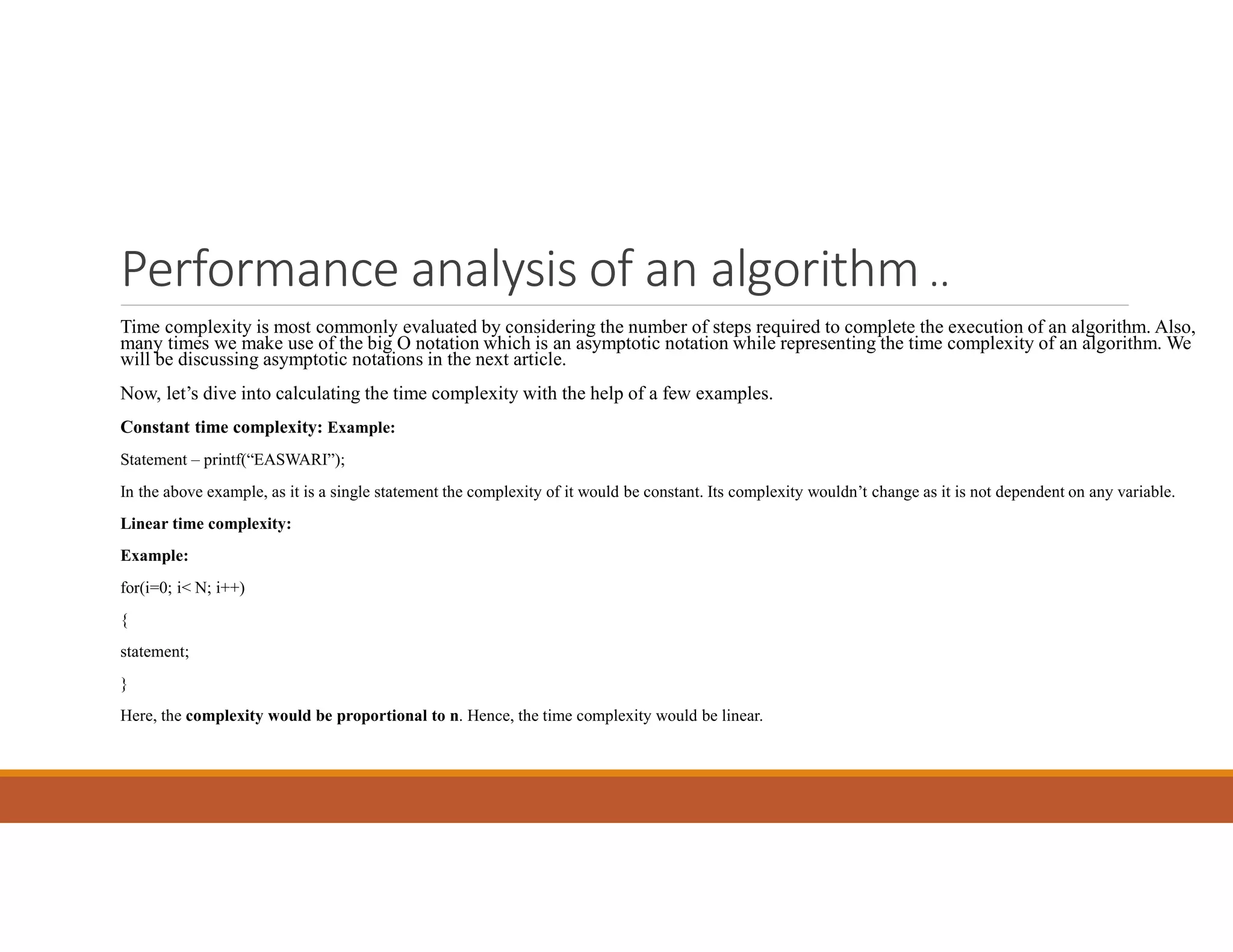
3. The time and space complexity of an algorithm measures how resources grow as the input size increases. Time complexity is evaluated based on the number of steps, while space complexity depends on memory usage. Common complexities include constant, linear, quadratic, and


![Performance analysis of an algorithm ..
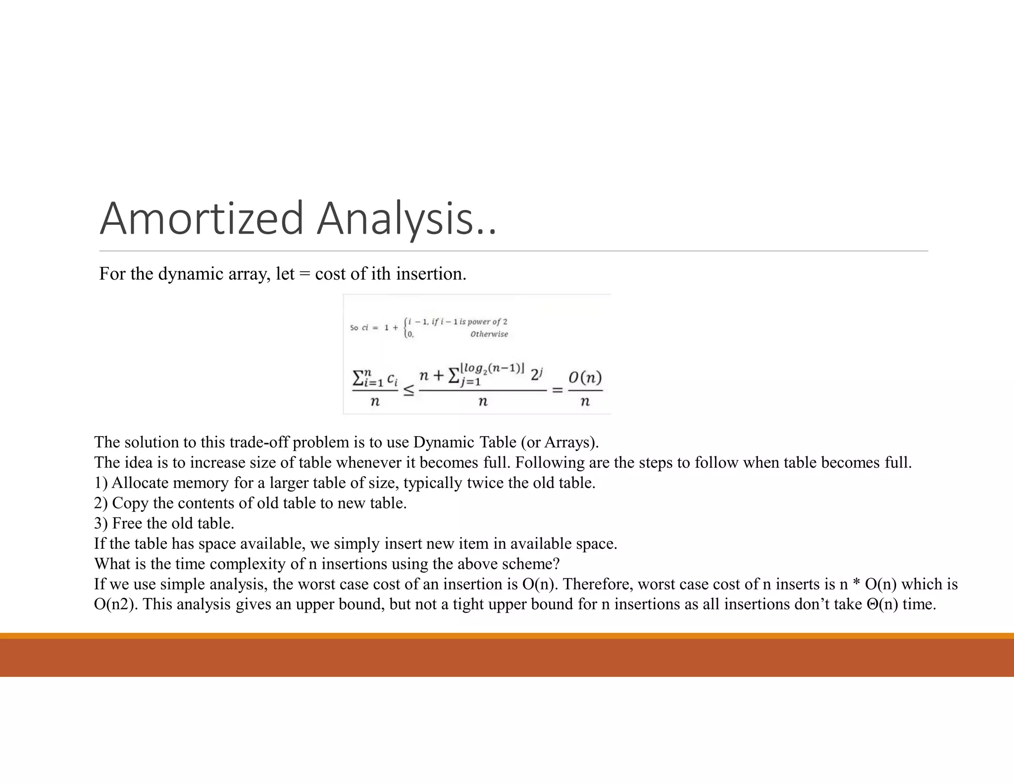
Logarithmic time complexity:
Example:
while(low <= high)
{
mid = (low + high) / 2;
if (target < list[mid])
high = mid - 1;
else if (target > list[mid])
low = mid + 1;
else break;
}
In this example, we are working on dividing a set of numbers into two parts. Which means that the complexity would be
proportional to the number of times n can be divided by 2, which is a logarithmic value. Hence we have a logarithmic time
complexity.](https://image.slidesharecdn.com/daaunit1-230222183709-88d2c90f/75/DAA-Unit-1-pdf-19-2048.jpg)
![Performance analysis of an algorithm ..
Example:1 Algorithm for Transpose of a Matrix
1. Create an auxiliary dummy_matrix that stores the transpose of the_matrix.
2. For a row in the first matrix, make it the first column in the newly constructed matrix.
3. Move to the next row and do it for all the rows. B[i][j] = A[j][i] , B is Transpose of A.
4. After completing all the rows, print the new_matrix, it is a Transpose of the given_matrix.
Time Complexity O(n2)
where n is the maximum of r1 and c1.
Here we simply run two loops first loop run r1 times and the second loop runs c1 times.
And inside the second loop, we just change the location of the current element in the auxiliary matrix.
Space Complexity O(m2)
where m is the maximum of r1 and c1.
Here we create extra space for storing the transpose of the given_matrix.
Here we also declared r1*c1 size for taking input from the given matrix.](https://image.slidesharecdn.com/daaunit1-230222183709-88d2c90f/75/DAA-Unit-1-pdf-20-2048.jpg)


![Probabilistic Analysis..
What is Indicator Random Variable?
It is a powerful technique that is used for computing the expected value of a random variable. Also, it is a convenient method for converting between
probabilities and also expectations. Indicator Random Variable takes only 2 values, which are 1 and 0.
Indicator Random Variable XA=I{A} for an event A of a sample space is defined as:
I{A} = 1 if A occurs
0 if A does not occur
The expected value of an indicator Random Variable is associated with an event A is equal to the probability that A occurs.
Indicator RV – Example
Problem: Determine the expected number of heads in one toss.
Sample space is s{H, T}
Indicator random variable
XA= I{ coin coming up with heads}=1/2
The expected number of heads obtained in one flip of the coin is equal to the expected value of the indicator random variable.
Therefore, E[XA] = 1/2
This is all about probabilistic analysis, Hiring problem, and the Indicator random variable. Do check the next article on Disjoint sets.](https://image.slidesharecdn.com/daaunit1-230222183709-88d2c90f/75/DAA-Unit-1-pdf-35-2048.jpg)