Downloaded 48 times


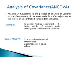
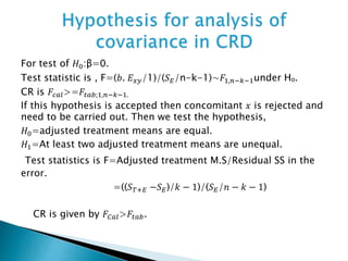
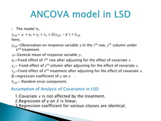
![ For test of 𝐻ₒ: 𝛽=0.
Test statistic is , F=[{(𝐸 𝑥𝑦)²/𝐸 𝑥𝑥}/1]/[𝑆 𝐸/{(𝑟 − 1)(𝑘 − 1) − 1}] under 𝐻ₒ.
CR is 𝐹𝑐𝑎𝑙>=𝐹𝑡𝑎𝑏;1, (𝑟 − 1)(𝑘 − 1) − 1.
If this hypothesis is accepted then concomitant 𝑥 is rejected and need
to be carried out . Then we test the hypothesis,
𝐻0=adjusted treatment means are equal.
𝐻1=At least two adjusted treatment means are unequal.
Test statistics is F=Adjusted treatment M.S/residual SS in the error.
=[(𝑆 𝑇+𝐸-𝑆 𝐸)/(𝑘 − 1)]/[𝑆 𝐸/(𝑟 − 1)(𝑘 − 1) − 1]
CR is given by 𝐹𝑐𝑎𝑙>𝐹𝑡𝑎𝑏.](https://image.slidesharecdn.com/split-plotdesignancovaandresponsesurfacedesign-190131144959/85/Basic-Concepts-of-Split-Plot-Design-Analysis-Of-Covariance-ANCOVA-Response-Surface-Design-Statistics-14-320.jpg)
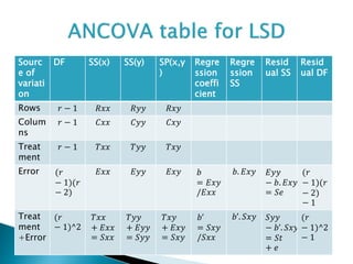
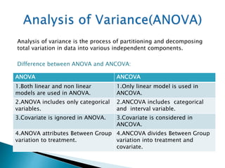
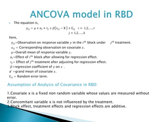
![ For test of 𝐻ₒ: 𝛽=0.
Test statistic is,F=[{(𝐸 𝑥𝑥)²/𝐸 𝑥𝑥}/1]/[𝑆 𝐸/{(𝑟 − 1)(𝑟 − 2) − 1}] under 𝐻ₒ.
CR is 𝐹𝑐𝑎𝑙>=𝐹𝑡𝑎𝑏;1, (𝑟 − 1)(𝑟 − 2) − 1.
,.If this hypothesis is accepted then concomitant 𝑥 is rejected and
need to be carried out . Then we test the hypothesis,
𝐻ₒ=adjusted treatment means are equal.
𝐻1=At least two adjusted treatment means are unequal.
Test statistics is F=Adjusted treatment M.S/residual SS in the
error.
=[(𝑆 𝑇+𝐸-𝑆 𝐸)/(𝑟 − 1)]/[𝑆 𝐸/(𝑟 − 1)(𝑟 − 2) − 1]
CR is given by 𝐹𝑐𝑎𝑙>𝐹𝑡𝑎𝑏.](https://image.slidesharecdn.com/split-plotdesignancovaandresponsesurfacedesign-190131144959/85/Basic-Concepts-of-Split-Plot-Design-Analysis-Of-Covariance-ANCOVA-Response-Surface-Design-Statistics-17-320.jpg)


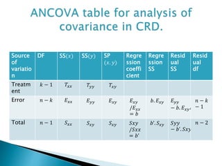
The document discusses various experimental design methods including split-plot design and analysis of covariance (ANCOVA), highlighting their applications, advantages, and disadvantages. It emphasizes the structure of these designs, providing mathematical models and examples, as well as the differences between ANOVA and ANCOVA. Additionally, it covers response surface methodology (RSM) for optimizing responses influenced by multiple variables.


![[Q1~12]Aclothingstoreisconsideringtwomethodstoreducetheselosses1).docx](https://cdn.slidesharecdn.com/ss_thumbnails/q112aclothingstoreisconsideringtwomethodstoreducetheselosses1-221114184210-53a9c855-thumbnail.jpg?width=640&height=640&fit=bounds)


![Lecture 5_Analysis of Variance [ANOVA].pptx](https://cdn.slidesharecdn.com/ss_thumbnails/lecture5analysisofvarianceanova-260107181555-9a697733-thumbnail.jpg?width=640&height=640&fit=bounds)


![제 23회 보아즈(BOAZ) 빅데이터 컨퍼런스 - [MBOAX] : ABSA를 활용한 소비자 반응 분석 기반 운영 효율화 대시보드 설계](https://cdn.slidesharecdn.com/ss_thumbnails/3-1boaz23rdconferencemboax-260203102709-9d519923-thumbnail.jpg?width=640&height=640&fit=bounds)


