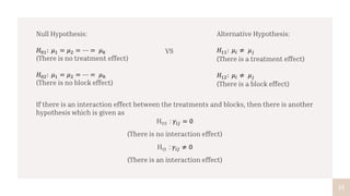
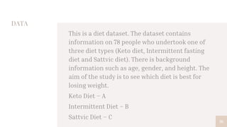
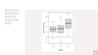
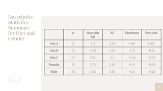
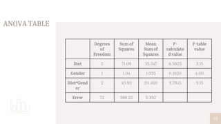
1. The document presents an analysis of a diet dataset containing information on 78 people who undertook one of three diets (Keto, Intermittent fasting, Sattvic) to analyze which diet is best for weight loss. 2. Descriptive statistics showed the Sattvic diet had the highest mean weight loss, while ANOVA results indicated diet type significantly affects weight loss but gender alone does not. 3. Post-hoc tests further revealed the Sattvic diet resulted in significantly more weight loss than the Keto or Intermittent fasting diets.

1. Diet
Vs
Weight-Loss
Analysis
DESIGNS OF EXPERIMENT PROJECT

2. Hello!
Presented by:
Vidit Jain - M013
75251219007
Our Mentor:
Prof. Preeti Ravikiran
2

3. “ Did you know “DIET”
stands for :
DID I EAT THAT?
3

4. Table of
Content
▫ Introduction
▫ Methodology
▫ Our Data
▫ Descriptive Statistics
▫ Proposed Hypothesis
▫ Test for Normality & Homogeneity of Variance
▫ Analysis of Variance (ANOVA)
▫ Conclusions
▫ Post –Hoc Tests
▫ Inferences
4

5. Designs of
Experiment
Designs of experiment (DOE) is defined as a
branch of applied statistics that deals with
planning, conducting, analyzing, and interpreting
tests to evaluate the factors that control the value
of a parameter or group of parameters. DOE is a
powerful data collection and analysis tool that
can be used in a variety of experimental
situations.
5

6. ANOVA
ANALYSIS OF VARIANCE

7. Analysis of variance (ANOVA) is a statistical technique that is used to check
if the means of two or more groups are significantly different from each
other. ANOVA checks the impact of one or more factors by comparing the
means of different samples.
7

8. ASSUMPTIONS
1. All effects are additive.
2. The observations are independent of each
other.
3. eij’s ∼ N(0, σ2)
4. The dependent variables should be
measurable.
5. Parent population from which samples are
drawn should be normal.
6. Homogeneity of variance between the groups
should be satisfied. 8

9. A test that allows one to make comparisons
between the means of three or more groups
of data, where one independent variables is
considered.
The one-way ANOVA model is given by,
𝑥𝑖𝑗 = 𝜇 + 𝛼𝑖 + 𝜖𝑖𝑗
Dependent variable = overall mean +
treatment effect + random error
9
One-Way ANOVA

10. 10
Null Hypothesis:
𝐻0: 𝜇1 = 𝜇2 = ⋯ = 𝜇𝑘
(There is no difference in the
population means)
VS
Alternative Hypothesis:
𝐻1: 𝜇𝑖 ≠ 𝜇𝑗
(At least two population
means are different)
TSS = SSTr + SSE
𝑇𝑆𝑆 = 𝑇𝑜𝑡𝑎𝑙 𝑆𝑢𝑚 𝑜𝑓 𝑆𝑞𝑢𝑎𝑟𝑒𝑠 =
𝑖 𝑗
(𝑥𝑖𝑗 − 𝑥. . )2
𝑆𝑆𝑇𝑟 = 𝑆𝑢𝑚 𝑜𝑓 𝑆𝑞𝑢𝑎𝑟𝑒𝑠 𝑑𝑢𝑒 𝑡𝑜 𝑇𝑟𝑒𝑎𝑡𝑚𝑒𝑛𝑡𝑠 =
𝑖 𝑗
(𝑥𝑖. −𝑥. . ) =
𝑖
𝑛𝑖( 𝑥𝑖. −𝑥. . )
𝑆𝑆𝐸 = 𝑆𝑢𝑚 𝑜𝑓 𝑆𝑞𝑢𝑎𝑟𝑒𝑠 𝑑𝑢𝑒 𝑡𝑜 𝐸𝑟𝑟𝑜𝑟𝑠 =
𝑖 𝑗
(𝑥𝑖𝑗 − 𝑥𝑖. )2

11. Source of
Variation
Sum of
Squared
Degree of
Freedom
Mean Sum
of Squares
Fcal Ftab
Treatment SSTr k-1 𝑀𝑆𝑆𝑇𝑟
=
𝑆𝑆𝑇𝑟
𝑘 − 1
𝐹
=
𝑀𝑆𝑆𝑇𝑟
𝑀𝑆𝑆𝐸
𝐹
𝛼(𝑘 − 1, 𝑁 − 𝑘)
Error SSE N-k 𝑀𝑆𝑆𝐸
=
𝑆𝑆𝐸
𝑁 − 𝑘
Total TSS N-1
11

12. A test that allows one to make comparisons
between the means of three or more groups of
data, where two independent variables are
considered.
The two-way ANOVA model is given by,
𝑥𝑖𝑗 = 𝜇 + 𝛼𝑖 + 𝛽𝑗 + 𝜖𝑖𝑗
Dependent variable = overall mean + treatment
effect + block effect + random error
12
Two Way ANOVA

13. 13
VS
Null Hypothesis:
𝐻01: 𝜇1 = 𝜇2 = ⋯ = 𝜇𝑘
(There is no treatment effect)
𝐻02: 𝜇1 = 𝜇2 = ⋯ = 𝜇ℎ
(There is no block effect)
Alternative Hypothesis:
𝐻11: 𝜇𝑖 ≠ 𝜇𝑗
(There is a treatment effect)
𝐻12: 𝜇𝑖 ≠ 𝜇𝑗
(There is a block effect)
If there is an interaction effect between the treatments and blocks, then there is another
hypothesis which is given as
H03 : 𝛾𝑖𝑗 = 0
(There is no interaction effect)
H13 : 𝛾𝑖𝑗 ≠ 0
(There is an interaction effect)

14. 14
Source of
Variation
Sum of
Squared
Degree of
Freedom
Mean Sum of
Squares
Fcal Ftab
Treatment SSTr p-1 𝑀𝑆𝑆𝑇𝑟
=
𝑆𝑆𝑇𝑟
𝑝 − 1
𝐹 =
𝑀𝑆𝑆𝑇𝑟
𝑀𝑆𝑆𝐸
𝐹
𝛼( 𝑝 − 1 , 𝑝𝑞(𝑚
Blocks SSB q-1
𝑀𝑆𝑆𝐵 =
𝑆𝑆𝐵
𝑞 − 1
𝐹 =
𝑀𝑆𝑆𝐵
𝑀𝑆𝑆𝐸
𝐹
𝛼( 𝑞 − 1 , 𝑝𝑞(𝑚
Interaction SSTr*B (p-1)(q-1) 𝑀𝑆𝑆𝑇𝑟 ∗ 𝐵
=
𝑆𝑆𝑇𝑟 ∗ 𝐵
(𝑝 − 1)(𝑞 − 1)
𝐹
=
𝑀𝑆𝑆𝑇𝑟 ∗ 𝐵
𝑀𝑆𝑆𝐸
𝐹
𝛼( 𝑝 − 1 (𝑞
Error SSE pq(m-1) 𝑀𝑆𝑆𝐸
=
𝑆𝑆𝐸
𝑚 − 1 𝑝𝑞
Total TSS Mpq-1

15. METHODOLOGY
1. Designing the experiment
2. Exploratory data analysis
3. Checking for normality
4. Homogeneity of variance
5. ANOVA
6. Conclusion
7. Inferences
15

16. DATA
This is a diet dataset. The dataset contains
information on 78 people who undertook one of
three diet types (Keto diet, Intermittent fasting
diet and Sattvic diet). There is background
information such as age, gender, and height. The
aim of the study is to see which diet is best for
losing weight.
Keto Diet – A
Intermittent Diet – B
Sattvic Diet – C
16

17. Descriptive
Statistics
Summary
for Diet and
Gender
17
n Mean (in
kg)
SD Skewness Kurtosis
Diet A 24 3.3 2.24 0.88 0.65
Diet B 27 3.03 2.52 -0.17 -0.74
Diet C 27 5.15 2.4 -0.34 -0.95
Female 45 3.72 2.59 0.01 -0.92
Male 33 4.02 2.53 0.12 -0.22

18. 18

19. BOX PLOT
SHOWING
WEIGHT
LOSS PER
DIET
19

20. HYPOTHESIS
H01 : 𝜇1 = 𝜇2
(There is no effect
of gender on weight
loss)
v/s
H11 : 𝜇𝑖 ≠ 𝜇𝑗
(There is an effect
of gender on weight
loss)
H02 : 𝜇1 = 𝜇2 = 𝜇3
(There is no effect
of diet type on
weight loss)
v/s
H12 : 𝜇𝑖 ≠ 𝜇𝑗
(There is an effect
of diet type on
weight loss)
H03 : 𝛾𝑖𝑗 = 0
(There is no
interaction effect
between gender
and diet)
v/s
H13 : 𝛾𝑖𝑗 ≠ 0
(There is an
interaction effect
between gender
and diet)
20

21. 21

22. TESTING
OUR DATA
FOR
NORMALITY
22
H0: The data is normally distributed Vs H1: The data is not
normally distributed
H0 is accepted

23. HOMOGENEITY
OF VARIANCE
23
H0: All groups have equal variance Vs H1: Variance of all
groups is not same
H0 is accepted

24. ANOVA TABLE
24
Degrees
of
Freedom
Sum of
Squares
Mean
Sum of
Squares
F-
calculate
d value
F-table
value
Diet 2 71.09 35.547 6.5925 3.15
Gender 1 1.04 1.035 0.1920 4.00
Diet*Gend
er
2 40.92 20.460 3.7945 3.15
Error 72 388.22 5.392

25. 25
CONCLUSION
Diet type Gender Interaction effect
H0 is rejected H0 is rejected
H0 is accepted

26. 1. Gender does not significantly affect average
weight loss.
2. Diet alone does not affect weight.
3. But combination of Gender and Diet has a
significant effect on weight loss.
26

27. 27

28. 28
t-value Degrees of
Freedom
p-value 95%
Confidence
Interval
A-B 0.40798 49 0.6851 (-1.075930,
1.624079)
A-C -2.8348 49 0.006644 (-3.1582988, -
0.5379975)
B-C -3.1693 52 0.00256 (-3.4658892, -
0.7785553)

29. Based on the Post Hoc
test, we can conclude
that Sattvic diet has a
significant effect.

30. 30
Weight loss
(Mean value)
t-value
Degrees of
Freedom p-value
95%
Confidence
Interval
Male female
Ketto Diet(A) 3.65 3.05 -0.6385 22 0.5297
(-2.548793,
0.1066417)
Intermittent
Diet(B) 2.28 4.11 -1.9460 25 0.06298
(-3.7923236,
0.1066417)
Sattvic Diet
( C) 4.23 5.88 1.8564 25 0.7522
(-0.1801614,
3.4734948)

31. ▫ Dieticians can use the result of this study to
analyse which diet is suitable for weight loss
for males and females.
▫ Further analysis can be done using the factors
age-group and diet.
31
FUTURE
SCOPE OF
THE STUDY

32. Thanks!
32