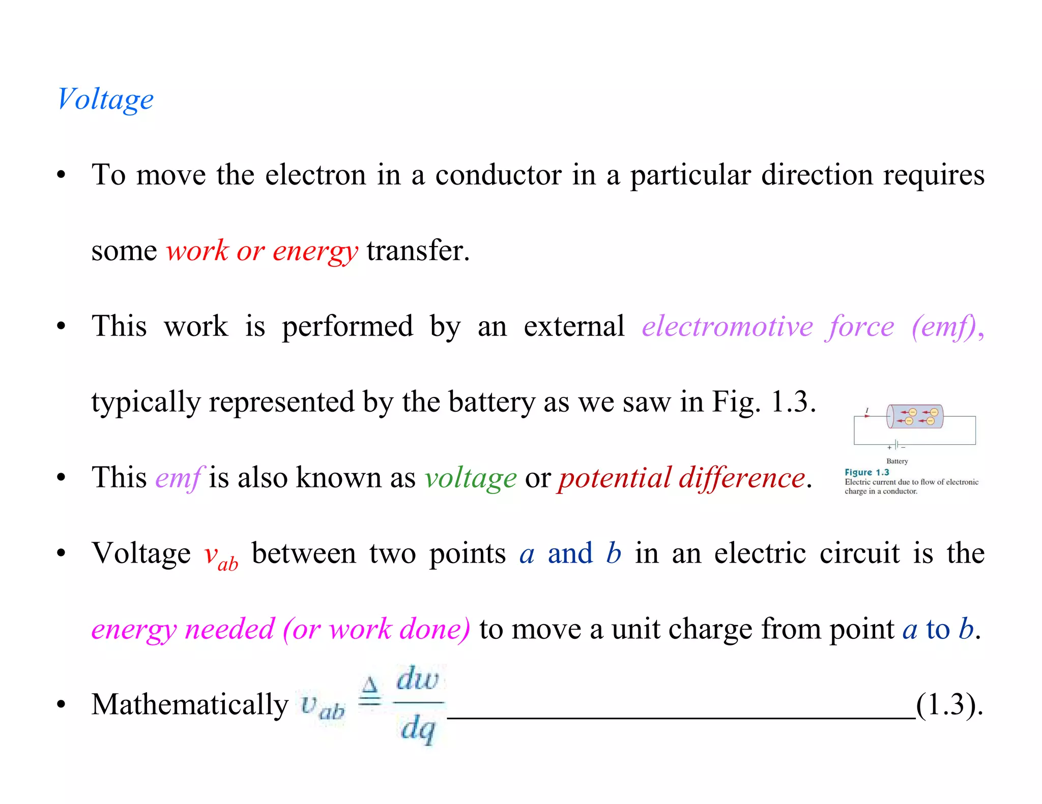
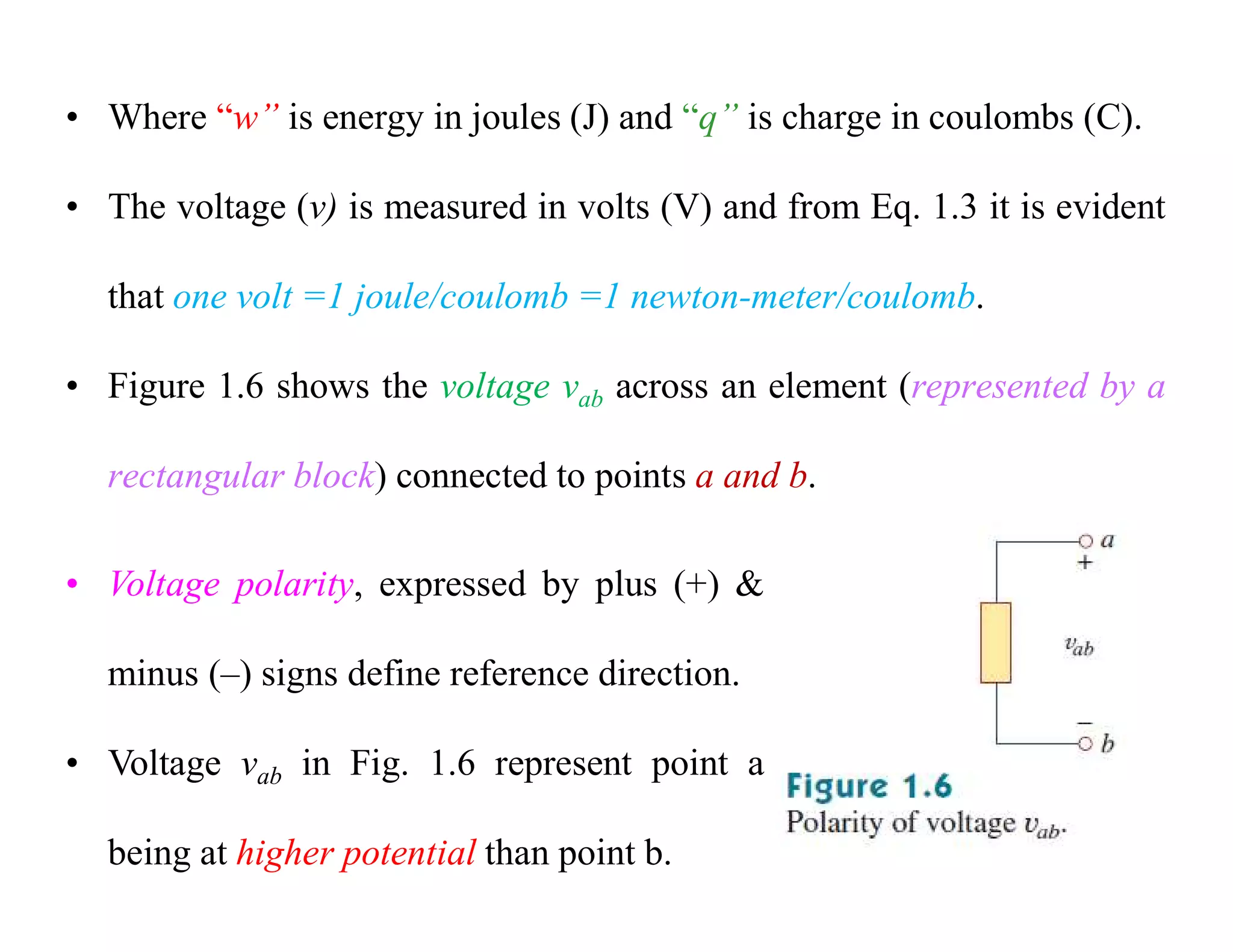
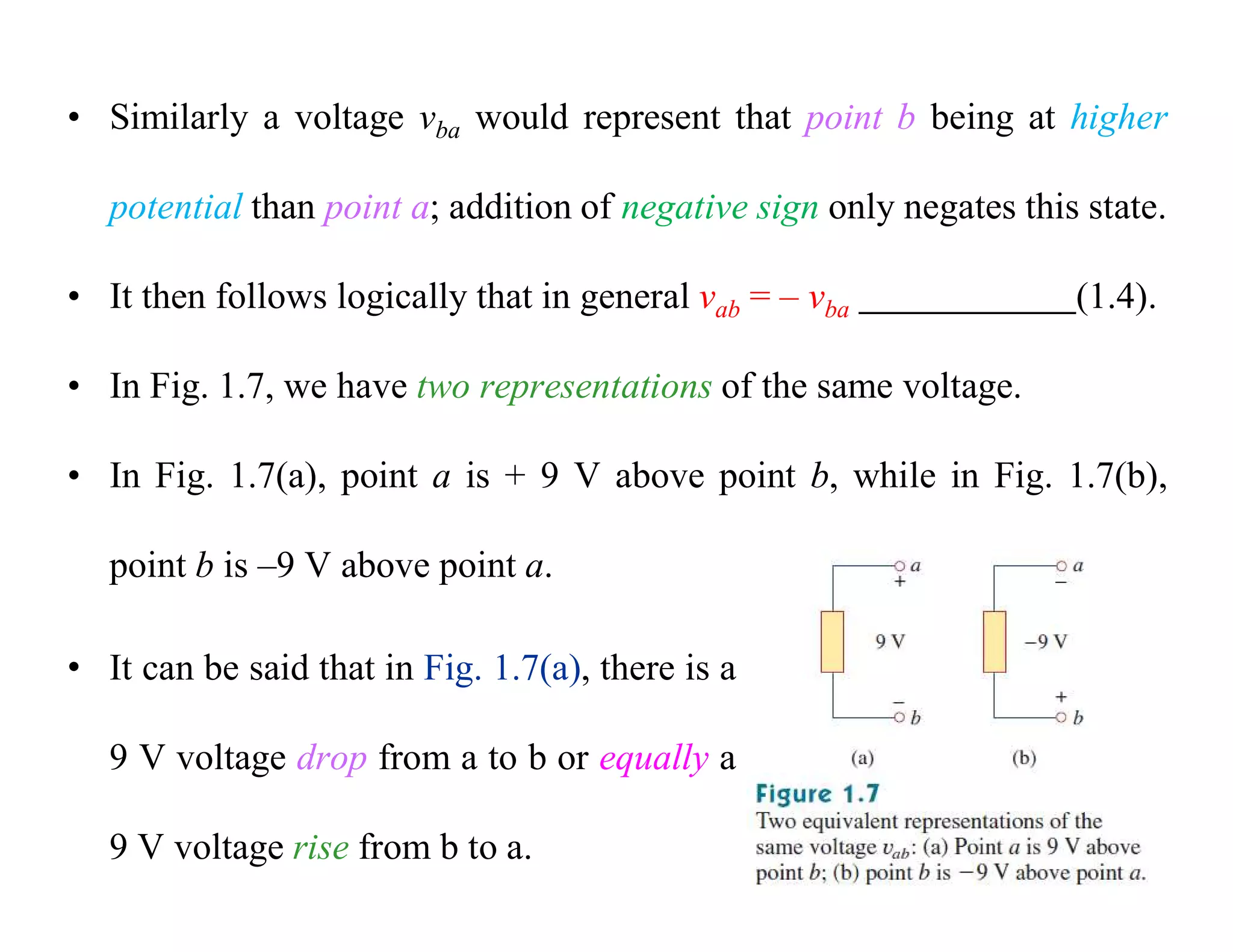
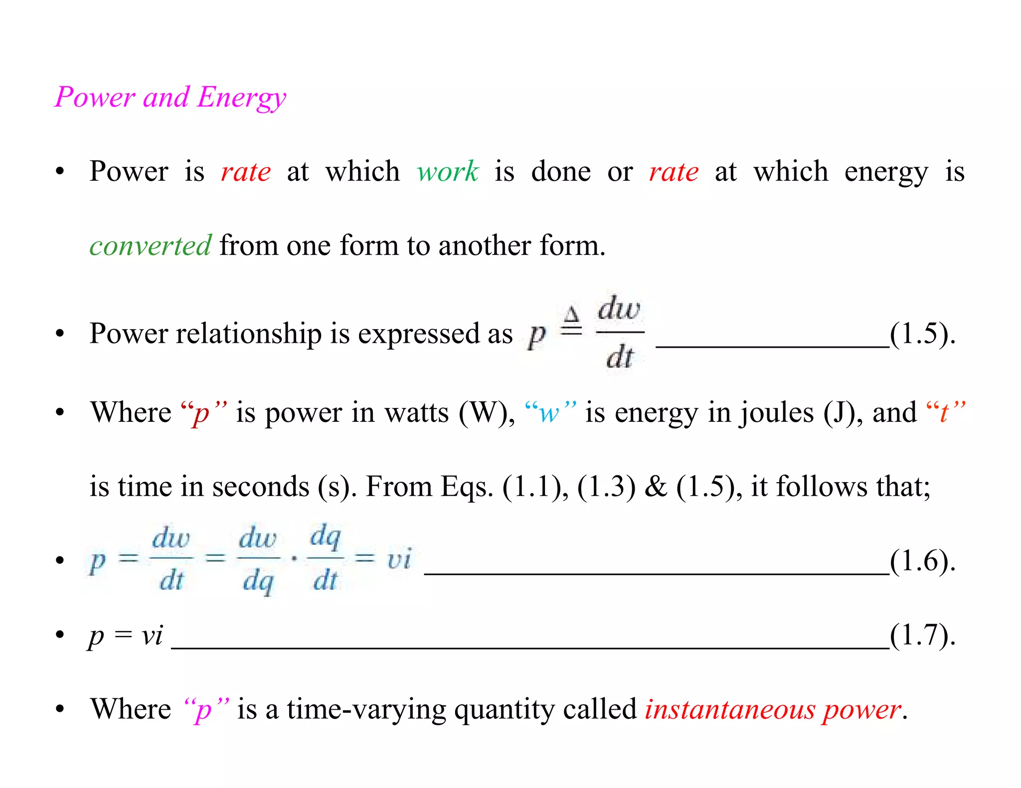
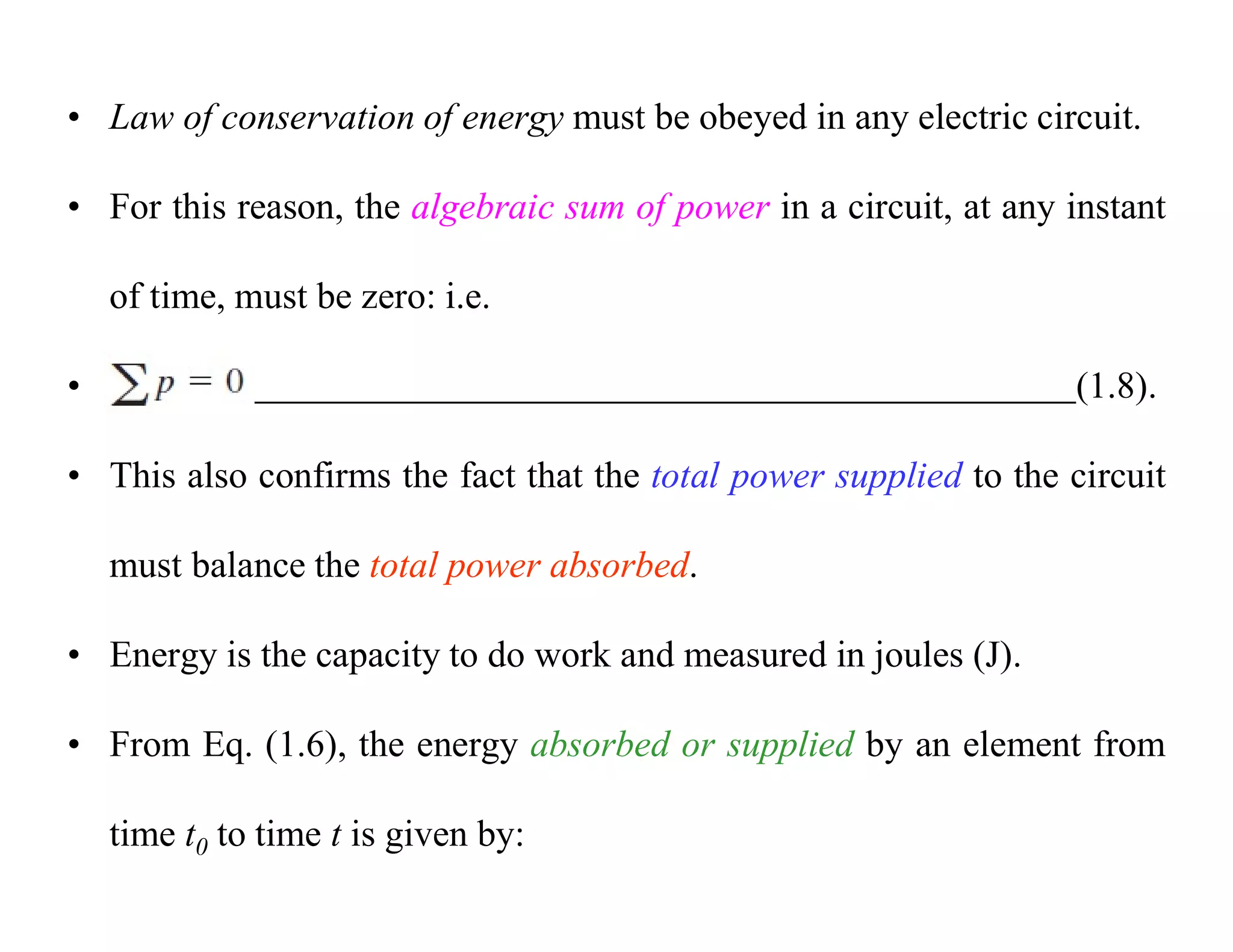
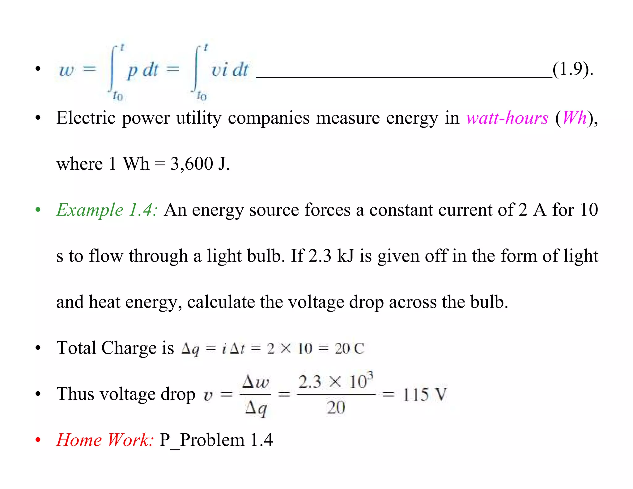
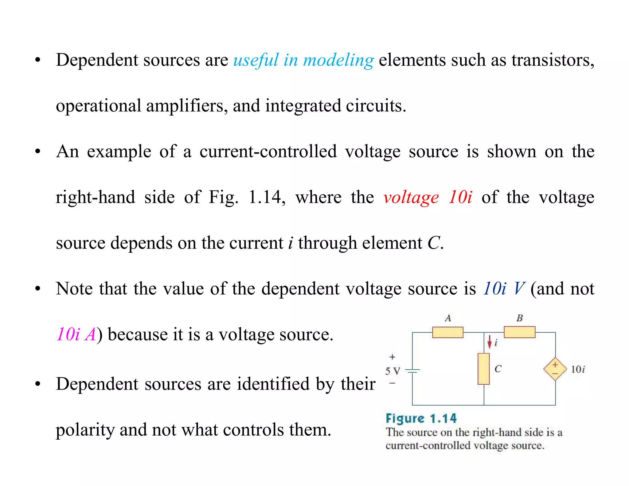
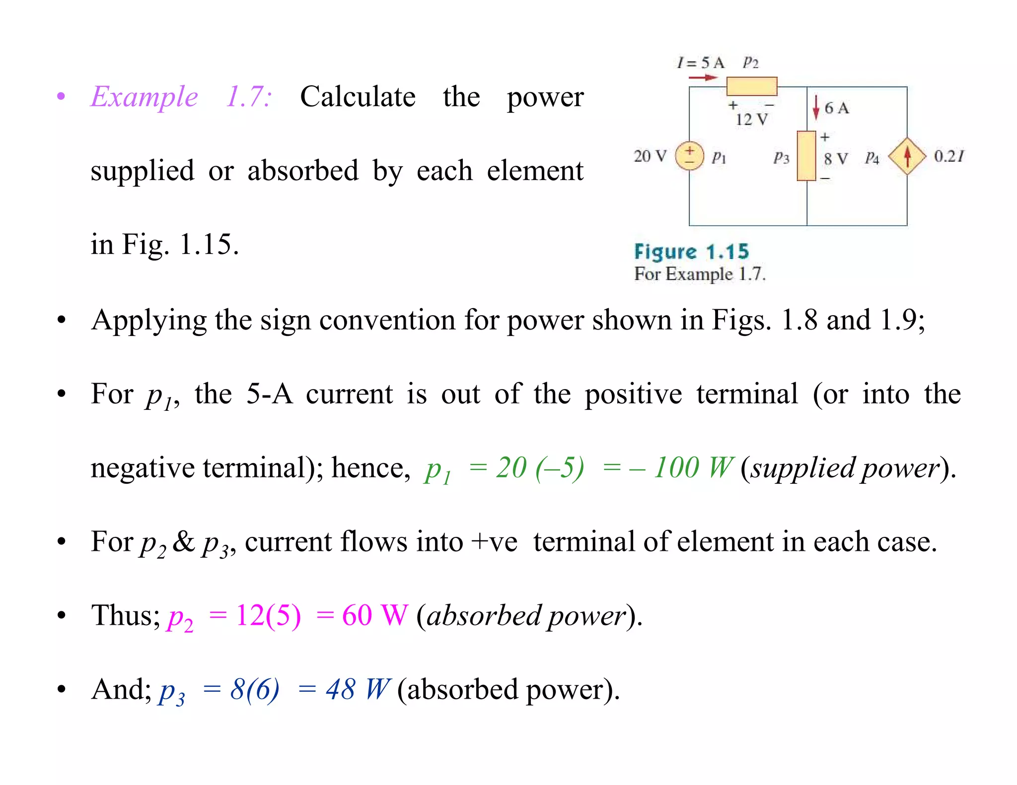
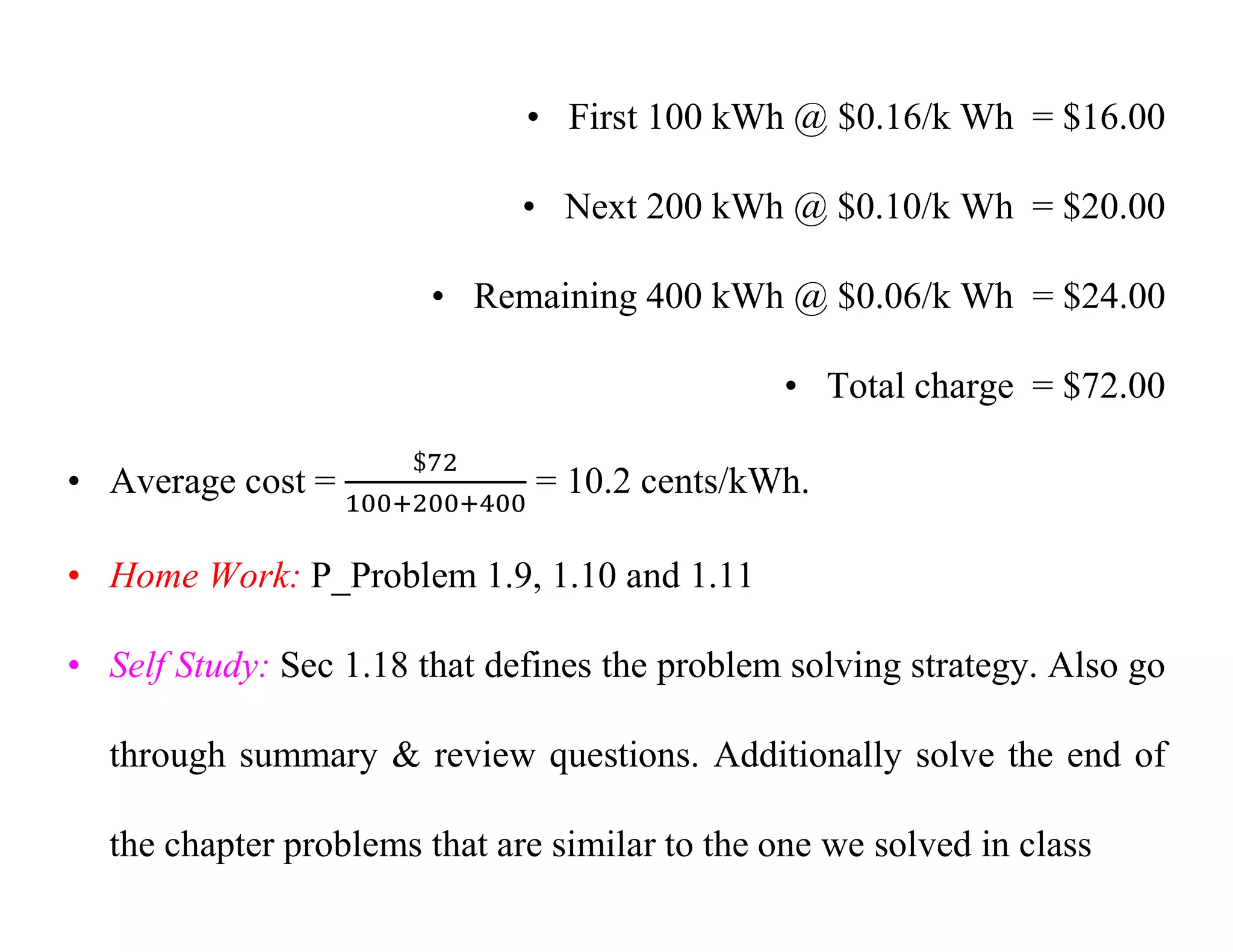
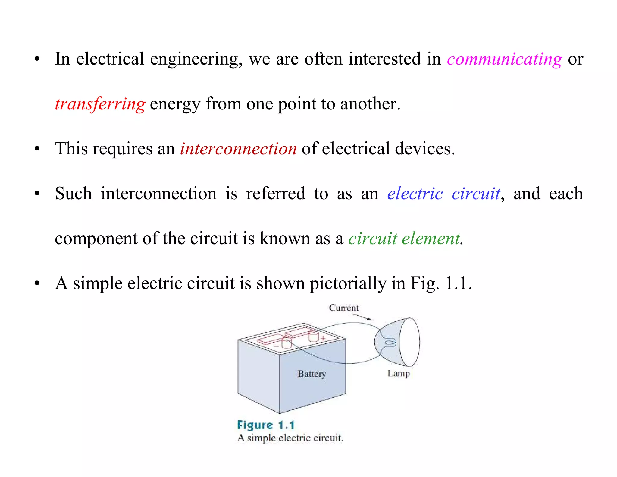
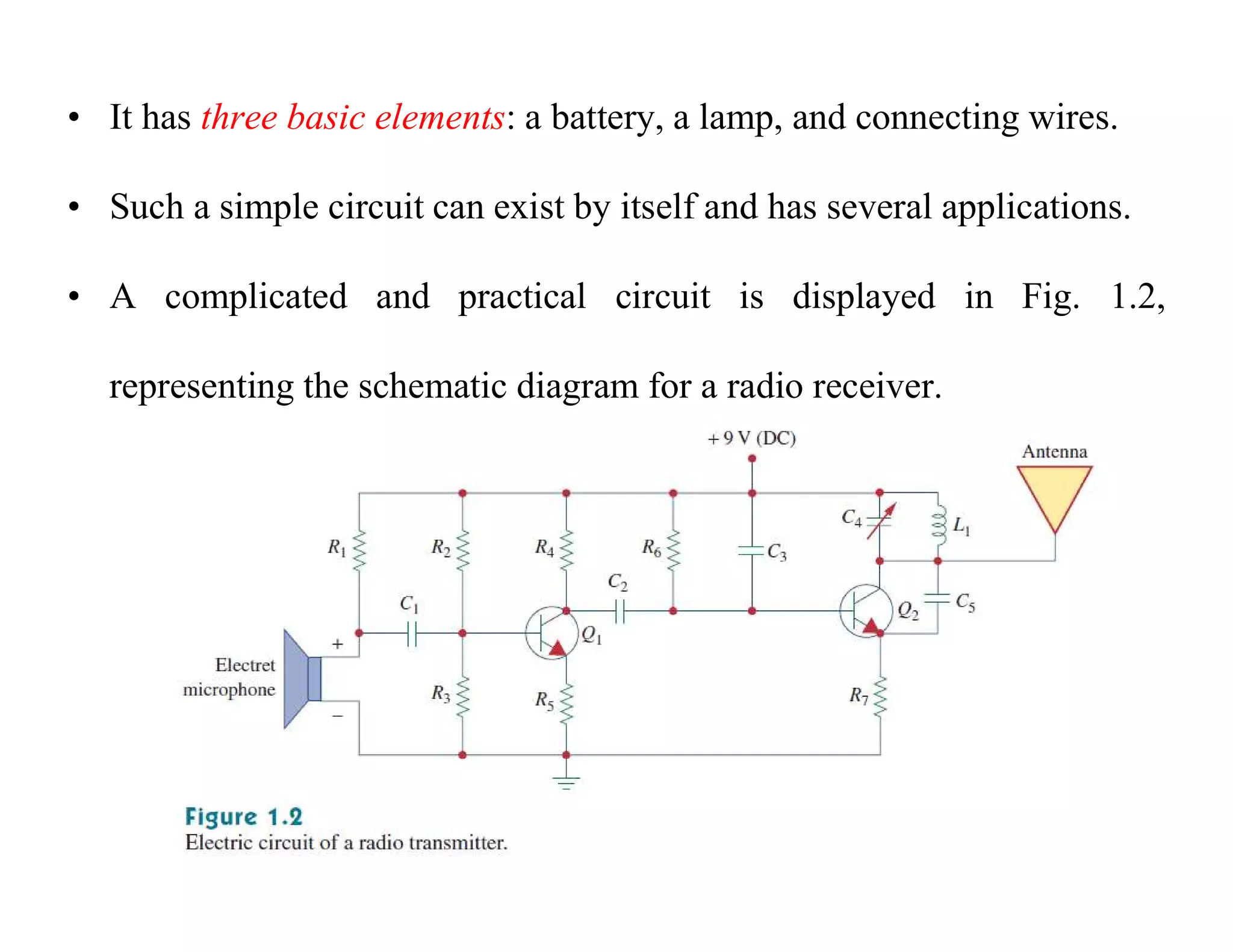
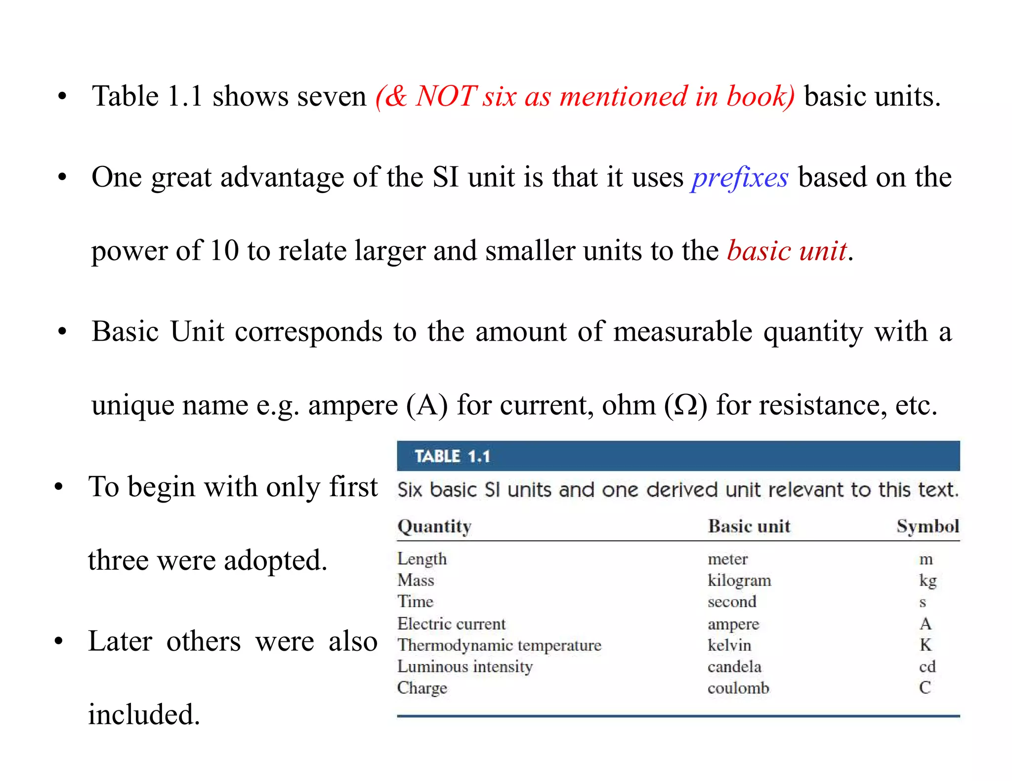
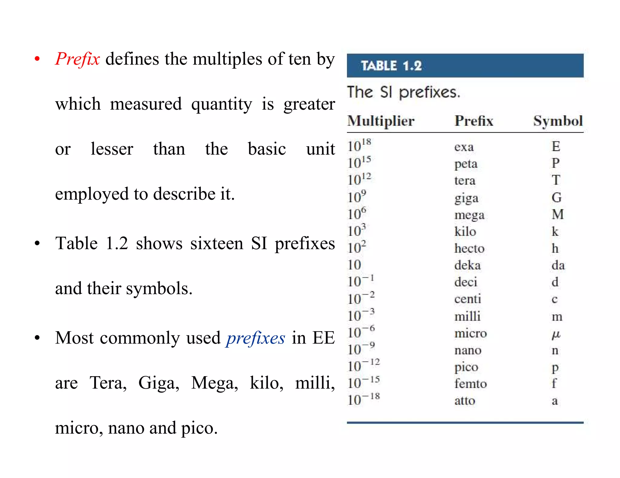
SlideShare a Scribd company logo
Chapter-1:Basic Concepts
1.1: Introduction
• Electric circuit and electromagnetic theory are the two fundamental
theories upon which all branches of electrical engineering are built.
• Many branches of electrical engineering, such as electric machines,
power, control, electronics, communications, and instrumentation, are
based on electric circuit theory.
• Therefore, the course like BEE that deals with basic electric circuit
theory is the most important course and always an excellent starting
point for initiating student of electrical engineering.
• In electrical engineering, we are often interested in communicating or
transferring energy from one point to another.
• This requires an interconnection of electrical devices.
• Such interconnection is referred to as an electric circuit, and each
component of the circuit is known as a circuit element.
• A simple electric circuit is shown pictorially in Fig. 1.1.
• It has three basic elements: a battery, a lamp, and connecting wires.
• Such a simple circuit can exist by itself and has several applications.
• A complicated and practical circuit is displayed in Fig. 1.2,
representing the schematic diagram for a radio receiver.
• Though it seems complicated, circuit of Fig. 1.2 can be analyzed using
the analysis techniques we plan to learn in this course.
• Our goal in this course is to learn various analytical techniques for
describing the behavior of a such like electrical circuits.
• Electric circuits are used in numerous electrical systems to accomplish
different tasks.
• Our objective in this course is NOT the study of various uses and
applications of circuits.
• Rather, our major concern will remain the analysis of the circuits.
• By the analysis of a circuit, we mean a study of the behavior of the
circuit i.e. how does it respond to a given input?
• How the interconnected elements and devices in the circuit interact?
• We commence our study by defining some basic concepts.
• These concepts include charge, current, voltage, circuit elements,
power, and energy.
• Before defining these concepts, we must first establish a system of
units that we will use throughout the course. Why we need it?
System of units
• Electrical engineers deal with measurable quantities that must be
communicated in a standard language so that it can be interpreted
universally through out the world.
• Such an international measurement language is the International
System of Units (or SI for brief), adopted by the General Conference
on Weights and Measures in 1960.
• In this system, there are seven principal units (mutually independent)
from which units of all other physical quantities can be derived.
• Table 1.1 shows seven (& NOT six as mentioned in book) basic units.
• One great advantage of the SI unit is that it uses prefixes based on the
power of 10 to relate larger and smaller units to the basic unit.
• Basic Unit corresponds to the amount of measurable quantity with a
unique name e.g. ampere (A) for current, ohm () for resistance, etc.
• To begin with only first
three were adopted.
• Later others were also
included.
• Prefix defines the multiples of ten by
which measured quantity is greater
or lesser than the basic unit
employed to describe it.
• Table 1.2 shows sixteen SI prefixes
and their symbols.
• Most commonly used prefixes in EE
are Tera, Giga, Mega, kilo, milli,
micro, nano and pico.
Charge and Current
• Most elementary quantity that we analyze in any electrical circuit is
charge. What is a an electric charge?
• Electric charge is a building block for electricity.
• What is electricity?
• Electricity is a form of energy i.e. the capacity to execute a work.
• Recall the difference between energy and work?
• Electric charge is inherited basic property of matter, occurs only in
discrete natural unit and can neither be created nor destroyed.
• Charge is found on sub-atomic particles such as electrons & protons.
• This charge on single electron or proton is refereed to as elementary
charge and is adopted as (– 1) for an electron and (+ 1) for a proton.
• It is the motion of charge in the circuit, which is responsible for
energy transfer among electrical components of electrical circuit.
• Basic unit of charge is Coulomb (C). One Coulomb of charge is
defined as the amount of charge possesses by 6.25 x 10¹⁸ electrons.
• An electron (& proton) thus possess 1/ 6.25 x 10¹⁸ C of charge that
translates into 1.6 x 10⁻¹⁹ coulombs i.e. elementary charge.
• Things that must be considered while analyzing a charge include:
1. Coulomb is a large unit for charges. The realistic or laboratory values
of charges are on the order of pC, nC, or µC.
2. Experimental observations reveal that charges occur only in nature
are integral multiples of the elementary charge i.e. 1.602 x 10⁻¹⁹ C
3. The law of conservation of charge states that charge can neither be
created nor destroyed, only transferred. Thus the algebraic sum of the
electric charges in a system does not change.
• We next consider the flow of electric charges.
• A unique feature of electric charge is the fact that it can be transferred
from one place to another through a medium.
• To do so an emf is needed to push the positive charges move in one
direction and negative charges in the opposite direction.
• This motion of charges creates electric current.
• Conventional current flow is based on movement of positive charges.
• That is, opposite to the flow of negative
charges, known as electronic current flow
as illustrated in Fig. 1.3.
• In this course we will follow the conventional current flow.
• Electric current is defined as the time rate of change of charge, and is
measured in amperes (A).
• Mathematically, relationship between current i, charge q, and time t is
given by (1.1).
• Current is measured in amperes (A), and 1A = 1C/1s.
• Charge transferred between time t0 and t is obtained by integrating
both sides of Eq. (1.1), which yields,
• (1.2).
• Current that does not change with time, but
remains constant, is called direct current.
• By convention the symbol (I) is used to
represent a constant current (dc).
• A time-varying current is represented by
the symbol (i).
• A common form of time-varying current is
the sinusoidal current called the
alternating current (ac). (See Fig.1.4)
• Once we define current as the movement of charge, we expect current
to have an associated direction of flow.
• As mentioned earlier, the direction of current flow is conventionally
taken as the direction of positive charge movement.
• Based on conventional current flow, a current of 5 A may be
represented positively or negatively as shown in Fig. 1.5.
• A –5 A current flowing in one direction
is the same as +5 A current flowing in
the opposite direction. (see Fig. 1.5)
• Example 1.1: How much charge is represented by 4,600 electrons?
• Each electron has –1.602 x 10⁻¹⁹ C charge on it, thus charge on 4600
electrons will be q = 4600 x –1.602 x 10⁻¹⁹ C = –7.369 x 10⁻¹⁶ C.
• Class Work: P_Problem 1.1; Calculate amount of charge represented
by six million protons. (6 x 10⁶)(1.602 x 10⁻¹⁹ C) = 9.612 x 10⁻¹³ C.
Example 1.2: For q = 5t sin 4t mC charge entering a terminal
calculate the current at t = 0.5?
• For i = = (5t sin 4 mC/s, applying chain rule differentiation
• i = [5 sin 4 t + (5t cos 4 t)(4 ] mA.
• i = [5 sin 4 t + 20 t cos 4 t] mA.
• And at t = 0.5;
• Home Work: P_Problem 1.2.
• Example 1.3: Determine the charge entering a terminal between t = 1s
to t = 2s if the current passing the terminal is i = (3t2 – t) A?
• and once solved,
• Q
• Home Work: P_Problem 1.3.
Voltage
• To move the electron in a conductor in a particular direction requires
some work or energy transfer.
• This work is performed by an external electromotive force (emf),
typically represented by the battery as we saw in Fig. 1.3.
• This emf is also known as voltage or potential difference.
• Voltage vab between two points a and b in an electric circuit is the
energy needed (or work done) to move a unit charge from point a to b.
• Mathematically (1.3).
• Where “w” is energy in joules (J) and “q” is charge in coulombs (C).
• The voltage (v) is measured in volts (V) and from Eq. 1.3 it is evident
that one volt =1 joule/coulomb =1 newton-meter/coulomb.
• Figure 1.6 shows the voltage vab across an element (represented by a
rectangular block) connected to points a and b.
• Voltage polarity, expressed by plus (+) &
minus (–) signs define reference direction.
• Voltage vab in Fig. 1.6 represent point a
being at higher potential than point b.
• Similarly a voltage vba would represent that point b being at higher
potential than point a; addition of negative sign only negates this state.
• It then follows logically that in general vab = – vba (1.4).
• In Fig. 1.7, we have two representations of the same voltage.
• In Fig. 1.7(a), point a is + 9 V above point b, while in Fig. 1.7(b),
point b is –9 V above point a.
• It can be said that in Fig. 1.7(a), there is a
9 V voltage drop from a to b or equally a
9 V voltage rise from b to a.
• In other words, a voltage drop from a to b is equivalent to a voltage
rise from b to a.
• Current and voltage are the two basic variables in electric circuits.
• Engineers prefer to call such variables signals rather than
mathematical functions of time.
• Like electric current, a constant voltage is called a dc voltage and is
represented by V, whereas a sinusoidally time-varying voltage is
called an ac voltage and is represented by v.
• A dc voltage is commonly produced by a battery; ac voltage is
produced by an electric generator
Power and Energy
• Power is rate at which work is done or rate at which energy is
converted from one form to another form.
• Power relationship is expressed as (1.5).
• Where “p” is power in watts (W), “w” is energy in joules (J), and “t”
is time in seconds (s). From Eqs. (1.1), (1.3) & (1.5), it follows that;
• (1.6).
• p = vi (1.7).
• Where “p” is a time-varying quantity called instantaneous power.
• Thus, power absorbed or supplied by an element is the product of the
voltage across the element and the current that flows through it.
• Once power has a (+) sign, then it is being delivered to or absorbed by
the element and power with (–) sign, is being supplied by the element.
• How do we know when the power has a negative or a positive sign?
• Current direction and voltage polarity play a major role in
determining the sign of power.
• Relationship between current i and voltage v in Fig. 1.8(a) provide the
reference polarities for power using the passive sign convention.
• By passive sign convention, for the power
to have a positive sign the voltage polarity
and current direction must conform with
those shown in Fig. 1.8(a).
• When, vi > 0 or p = +vi, it implies that element is absorbing power.
• However, if p = –vi or vi < 0 , as in Fig. 1.8(b), then the element is
supplying the power.
• Unless otherwise stated, we will follow the passive sign convention
throughout this course.
• For example, element in both circuits of
Fig. 1.9 has an absorbing power of 12 W
because a positive current enters the
positive terminal in both cases.
• In Fig. 1.10, however, both elements are
supplying 12 W power because a positive
current enters the negative terminal.
• Simple assigning of positive or negative
sign to power also convey same status.
• Law of conservation of energy must be obeyed in any electric circuit.
• For this reason, the algebraic sum of power in a circuit, at any instant
of time, must be zero: i.e.
• (1.8).
• This also confirms the fact that the total power supplied to the circuit
must balance the total power absorbed.
• Energy is the capacity to do work and measured in joules (J).
• From Eq. (1.6), the energy absorbed or supplied by an element from
time t0 to time t is given by:
• (1.9).
• Electric power utility companies measure energy in watt-hours (Wh),
where 1 Wh = 3,600 J.
• Example 1.4: An energy source forces a constant current of 2 A for 10
s to flow through a light bulb. If 2.3 kJ is given off in the form of light
and heat energy, calculate the voltage drop across the bulb.
• Total Charge is
• Thus voltage drop
• Home Work: P_Problem 1.4
• Example 1.5: Find the power delivered to an element at t = 3 ms if the
current entering its positive terminal is i = 5 cos 60  t A and the
voltage is: (a) v = 3i, (b) v = 3 di/dt.
(a) The voltage is v = 3i = 15 cos 60  t; hence, the power is
• p = vi = 75 cos2 60  t W.
• At t = 3 ms, p = 75 cos2 (60  0.003) = 75 cos2 0.18  = 53.48 W.
(b) We find the voltage and the power as
•
• p = vi = – 4500  sin 60  t cos 60  t W
• At t = 3 ms, p = vi = – 4500  sin 60  0.003 cos 60  0.003 W
• p = vi = – 4500  sin 0.18  cos 0.18  W, and once solved,
• p = –14137.167 sin 32.4 cos 32.4 = – 6.396 kW. (energy supplied)
• Home Work: P_Problem 1.5
• Example 1.6: How much energy does a 100-W electric bulb consume
in two hours?
• w = pt = 100 (W) x 2 (h) x 60 (min/h) x 60 (s/min)
• w = pt = 720,000 J = 720 kJ
• This is same as, w = pt = 100 W x 2 h = 200 Wh
• Home Work: P_Problem 1.6
Circuit Elements
• An element is the basic building block of a circuit and an electric
circuit is simply an interconnection of the elements.
• Circuit analysis is the process of determining voltages across (or the
currents through) the elements of the circuit.
• There are two types of elements found in electric circuits: passive
elements and active elements. Passive elements absorb energy.
• Examples of passive elements are resistors, capacitors, and inductors.
• Active element can generating energy (while passive element can’t).
• Typical active elements include generators, batteries, operational
amplifiers, solar panels, fuel cells etc.
• The most important active elements are voltage or current sources that
generally deliver power to the circuit connected to them.
• There are two kinds of sources: independent and dependent sources.
• An ideal independent source provides a specified voltage or current
that is completely independent of other circuit elements.
• In other words, an ideal independent voltage source delivers to the
circuit whatever current is necessary to maintain its terminal voltage.
• Physical sources such as batteries and generators may be regarded as
approximations to ideal voltage sources.
• Figure 1.11 shows the symbols for independent voltage sources.
• Notice that both symbols in Fig. 1.11(a) and (b) can be used to
represent a dc voltage source, but only the symbol in Fig. 1.11(a) can
be used for a time-varying voltage source.
• An ideal independent current source
provides a specified current completely
independent of voltage across the source.
• In other words, the current source delivers to the circuit whatever
voltage is necessary to maintain the designated current.
• The symbol for an independent current source is displayed in Fig.
1.12, where the arrow indicates the direction of current i.
• Dependent sources are usually designated by diamond-shaped
symbols, as shown in Fig. 1.13.
• An ideal dependent (or controlled) source is an active element in
which the source output is controlled by another voltage or current.
• Since the control of the dependent source is achieved by a voltage or
current of some other element in the circuit, it follows that there are
four possible types of dependent sources, namely:
1. A voltage-controlled voltage source (VCVS).
2. A current-controlled voltage source (CCVS).
3. A voltage-controlled current source (VCCS).
4. A current-controlled current source (CCCS).
• Dependent sources are useful in modeling elements such as transistors,
operational amplifiers, and integrated circuits.
• An example of a current-controlled voltage source is shown on the
right-hand side of Fig. 1.14, where the voltage 10i of the voltage
source depends on the current i through element C.
• Note that the value of the dependent voltage source is 10i V (and not
10i A) because it is a voltage source.
• Dependent sources are identified by their
polarity and not what controls them.
• Ideal voltage source (dependent or independent) will always produce
any current required to ensure that the terminal voltage stays as stated,
• Similarly an ideal current source will produce the necessary voltage
required to ensure that the current always flows at stated magnitude.
• Thus, an ideal source could in theory supply an infinite energy.
• However it should be noted that not only do sources supply power to a
circuit, they can be configured to absorb power as well.
• For a voltage source, we know the voltage but not the current supplied
or drawn by it. By the same token, we know the current supplied by a
current source but not the voltage across it
• Example 1.7: Calculate the power
supplied or absorbed by each element
in Fig. 1.15.
• Applying the sign convention for power shown in Figs. 1.8 and 1.9;
• For p1, the 5-A current is out of the positive terminal (or into the
negative terminal); hence, p1 = 20 (–5) = – 100 W (supplied power).
• For p2 & p3, current flows into +ve terminal of element in each case.
• Thus; p2 = 12(5) = 60 W (absorbed power).
• And; p3 = 8(6) = 48 W (absorbed power).
• For p4, the voltage cross the dependent current source is 8 V (positive
at the top) and hence the current flows out of the positive terminal.
• Therefore, p4 = 8(– 0.2I ) = 8(– 0.2 x 5) = – 8 W (supplied power).
• Notice that the 20-V independent voltage source and 0.2I dependent
current source are supplying power to the rest of the network, while
the two passive elements are absorbing power.
• Also, in agreement with Eq. (1.8), the total power supplied equals the
total power absorbed i.e. p1 + p2 + p3 + p4 = – 100 + 60 + 48 – 8 = 0.
• Home Work: P_Problem 1.7 7 Problem 1.20 at the end of Chapter-1.
Applications
• The book explains two practical applications of the concepts
developed in chapter-1.
• The first one deals with the TV picture tube and the other with how
electric utilities determine electric bill.
• Students can learn the working of TV tube, if interested, as self study.
• The second application deals with how an electric utility company
charges their customers.
• The cost of electricity depends upon the amount of energy consumed
in kilowatt-hours (kWh). (other factors will be ignored for now).
• Note that, even if a consumer uses no energy at all, there is a
minimum service charge the customer must pay because it costs
money to stay connected to the power line.
• As energy consumption increases, the cost per kWh drops.
• It is interesting to note the average monthly consumption of household
appliances for a typical USA family of five, as shown in Table 1.3.
• Example 1.9: A homeowner consumes 700 kWh in January.
Determine the electricity bill for the month using the following
residential rate schedule?
 Base monthly charge of $12.00.
 First 100 kWh per month at 16 cents/kWh.
 Next 200 kWh per month at 10 cents/kWh.
 Over 300 kWh per month at 6 cents/kWh.
• We calculate the electricity bill as follows.
• Base monthly charge = $12.00
• First 100 kWh @ $0.16/k Wh = $16.00
• Next 200 kWh @ $0.10/k Wh = $20.00
• Remaining 400 kWh @ $0.06/k Wh = $24.00
• Total charge = $72.00
• Average cost = = 10.2 cents/kWh.
• Home Work: P_Problem 1.9, 1.10 and 1.11
• Self Study: Sec 1.18 that defines the problem solving strategy. Also go
through summary & review questions. Additionally solve the end of
the chapter problems that are similar to the one we solved in class

More Related Content

What's hot

Symmetrical components
Symmetrical componentsSymmetrical components
Symmetrical components
Sirat Mahmood
 
Electrical engineering, students notes
Electrical engineering, students notesElectrical engineering, students notes
Electrical engineering, students notes
IYAKAREMYE Jean De Dieu
 
Electric circuits-chapter-1 Basic Concept
Electric circuits-chapter-1 Basic ConceptElectric circuits-chapter-1 Basic Concept
Electric circuits-chapter-1 Basic Conceptrahman84
 
Electric circuits-chapter-2 Basic Laws
Electric circuits-chapter-2 Basic LawsElectric circuits-chapter-2 Basic Laws
Electric circuits-chapter-2 Basic Lawsrahman84
 
basic electronics
basic electronicsbasic electronics
basic electronics
ATTO RATHORE
 
ppt on Introduction to basic electrical concept by harshid panchal
ppt on Introduction to basic electrical concept by harshid panchalppt on Introduction to basic electrical concept by harshid panchal
ppt on Introduction to basic electrical concept by harshid panchal
harshid panchal
 
Chapter 4 mechanical design of transmission lines
Chapter 4  mechanical design of transmission linesChapter 4  mechanical design of transmission lines
Chapter 4 mechanical design of transmission lines
firaoltemesgen1
 
Classification of power supply and its different types
Classification of power supply and its different typesClassification of power supply and its different types
Classification of power supply and its different types
elprocus
 
PERFORMANCE OF TRANSMISSION LINES:
PERFORMANCE OF TRANSMISSION LINES:PERFORMANCE OF TRANSMISSION LINES:
PERFORMANCE OF TRANSMISSION LINES:
Duddu Rajesh
 
Electric network theorems
Electric network theoremsElectric network theorems
Electric network theorems
Mohsin Mulla
 
Electrical Circuit Analysis Ch 01 basic concepts
Electrical Circuit Analysis Ch 01 basic conceptsElectrical Circuit Analysis Ch 01 basic concepts
Electrical Circuit Analysis Ch 01 basic concepts
Ali Farooq
 
Kirchhoff's laws With Examples
Kirchhoff's laws With ExamplesKirchhoff's laws With Examples
Kirchhoff's laws With Examples
Muhammad Waqas
 
Linear circuit analysis 1
Linear circuit analysis 1Linear circuit analysis 1
Linear circuit analysis 1
Talha Mughal
 
Step respponse of rlc circuit by Aditya Pratap Singh Delhi University
Step respponse of rlc circuit by Aditya Pratap Singh Delhi UniversityStep respponse of rlc circuit by Aditya Pratap Singh Delhi University
Step respponse of rlc circuit by Aditya Pratap Singh Delhi University
Aditya Pratap Singh
 
Ac fundamentals
Ac fundamentalsAc fundamentals
Ac fundamentals
Anu71
 
Printed circuit board
Printed circuit boardPrinted circuit board
Printed circuit board
Suhail Ahmed
 
Circuit Analysis – DC Circuits
Circuit Analysis – DC CircuitsCircuit Analysis – DC Circuits
Circuit Analysis – DC Circuits
Vesa Linja-aho
 
Electrical engineering principles lecture slides. circuit analysis by Maina
Electrical engineering principles lecture slides. circuit analysis by MainaElectrical engineering principles lecture slides. circuit analysis by Maina
Electrical engineering principles lecture slides. circuit analysis by Maina
sylvand
 

What's hot (20)

Circuit Analysis-
Circuit Analysis-Circuit Analysis-
Circuit Analysis-
 
Symmetrical components
Symmetrical componentsSymmetrical components
Symmetrical components
 
Electrical engineering, students notes
Electrical engineering, students notesElectrical engineering, students notes
Electrical engineering, students notes
 
Electric circuits-chapter-1 Basic Concept
Electric circuits-chapter-1 Basic ConceptElectric circuits-chapter-1 Basic Concept
Electric circuits-chapter-1 Basic Concept
 
Electric circuits-chapter-2 Basic Laws
Electric circuits-chapter-2 Basic LawsElectric circuits-chapter-2 Basic Laws
Electric circuits-chapter-2 Basic Laws
 
basic electronics
basic electronicsbasic electronics
basic electronics
 
ppt on Introduction to basic electrical concept by harshid panchal
ppt on Introduction to basic electrical concept by harshid panchalppt on Introduction to basic electrical concept by harshid panchal
ppt on Introduction to basic electrical concept by harshid panchal
 
Chapter 4 mechanical design of transmission lines
Chapter 4  mechanical design of transmission linesChapter 4  mechanical design of transmission lines
Chapter 4 mechanical design of transmission lines
 
Classification of power supply and its different types
Classification of power supply and its different typesClassification of power supply and its different types
Classification of power supply and its different types
 
PERFORMANCE OF TRANSMISSION LINES:
PERFORMANCE OF TRANSMISSION LINES:PERFORMANCE OF TRANSMISSION LINES:
PERFORMANCE OF TRANSMISSION LINES:
 
Electric network theorems
Electric network theoremsElectric network theorems
Electric network theorems
 
Electrical Circuit Analysis Ch 01 basic concepts
Electrical Circuit Analysis Ch 01 basic conceptsElectrical Circuit Analysis Ch 01 basic concepts
Electrical Circuit Analysis Ch 01 basic concepts
 
Kirchhoff's laws With Examples
Kirchhoff's laws With ExamplesKirchhoff's laws With Examples
Kirchhoff's laws With Examples
 
Linear circuit analysis 1
Linear circuit analysis 1Linear circuit analysis 1
Linear circuit analysis 1
 
Step respponse of rlc circuit by Aditya Pratap Singh Delhi University
Step respponse of rlc circuit by Aditya Pratap Singh Delhi UniversityStep respponse of rlc circuit by Aditya Pratap Singh Delhi University
Step respponse of rlc circuit by Aditya Pratap Singh Delhi University
 
Ac fundamentals
Ac fundamentalsAc fundamentals
Ac fundamentals
 
Printed circuit board
Printed circuit boardPrinted circuit board
Printed circuit board
 
Circuit Analysis – DC Circuits
Circuit Analysis – DC CircuitsCircuit Analysis – DC Circuits
Circuit Analysis – DC Circuits
 
Electrical engineering principles lecture slides. circuit analysis by Maina
Electrical engineering principles lecture slides. circuit analysis by MainaElectrical engineering principles lecture slides. circuit analysis by Maina
Electrical engineering principles lecture slides. circuit analysis by Maina
 
mesh analysis
mesh analysismesh analysis
mesh analysis
 

Similar to Basic concepts linear circuit analysis

Chapter 1: Introduction to Principles of Electric and Electronics
Chapter 1: Introduction to Principles of Electric and ElectronicsChapter 1: Introduction to Principles of Electric and Electronics
Chapter 1: Introduction to Principles of Electric and Electronics
JeremyLauKarHei
 
Unit 1.doc
Unit 1.docUnit 1.doc
Unit 1.doc
T Srihari
 
Analysing Electric Fields and Charge Flow
Analysing Electric Fields and Charge FlowAnalysing Electric Fields and Charge Flow
Analysing Electric Fields and Charge Flow
Tuisyen Geliga
 
circuit analysis.pptx
circuit analysis.pptxcircuit analysis.pptx
circuit analysis.pptx
HendIbrahim35
 
1_Basic_Electricity-5.pptx
1_Basic_Electricity-5.pptx1_Basic_Electricity-5.pptx
1_Basic_Electricity-5.pptx
rutheliezeralcazar1
 
1_Basic_Electricity-5.pptx
1_Basic_Electricity-5.pptx1_Basic_Electricity-5.pptx
1_Basic_Electricity-5.pptx
YousabJacob
 
Basic-Electricity.pptx
Basic-Electricity.pptxBasic-Electricity.pptx
Basic-Electricity.pptx
DrMSAli1
 
1_Basic_Electricity-5.pptx
1_Basic_Electricity-5.pptx1_Basic_Electricity-5.pptx
1_Basic_Electricity-5.pptx
TahaSaquib1
 
electronics fundamental of dc and ac circits.pdf
electronics fundamental of dc and ac circits.pdfelectronics fundamental of dc and ac circits.pdf
electronics fundamental of dc and ac circits.pdf
RamaSaiJahnavi
 
Lecture 1 & 2.pdf
Lecture 1 & 2.pdfLecture 1 & 2.pdf
Lecture 1 & 2.pdf
Athar Baig
 
Exp SPA - Chp 17 Current of Electricity
Exp SPA - Chp 17 Current of ElectricityExp SPA - Chp 17 Current of Electricity
Exp SPA - Chp 17 Current of Electricity
harrywwh
 
B tech ee ii_ eee_ u-1_ dc circuit analysis_dipen patel
B tech ee  ii_ eee_ u-1_ dc circuit analysis_dipen patelB tech ee  ii_ eee_ u-1_ dc circuit analysis_dipen patel
B tech ee ii_ eee_ u-1_ dc circuit analysis_dipen patel
Rai University
 
IGCSE-CL10-CH 18-ELEC QTTIES.pptx
IGCSE-CL10-CH 18-ELEC QTTIES.pptxIGCSE-CL10-CH 18-ELEC QTTIES.pptx
IGCSE-CL10-CH 18-ELEC QTTIES.pptx
RachnaRishi2
 
Diploma i boee u 2 dc circuit analysis
Diploma i boee u 2 dc circuit analysisDiploma i boee u 2 dc circuit analysis
Diploma i boee u 2 dc circuit analysis
Rai University
 
Unit 1 _Basics of electrical system.pptx
Unit 1 _Basics of electrical system.pptxUnit 1 _Basics of electrical system.pptx
Unit 1 _Basics of electrical system.pptx
Jaya Singh
 
Lesson plan physics class 10 introduction to electric current
Lesson plan physics class 10 introduction to electric currentLesson plan physics class 10 introduction to electric current
Lesson plan physics class 10 introduction to electric current
International advisers
 
Electrical circuitsand methods of network analysis
Electrical circuitsand methods of network analysisElectrical circuitsand methods of network analysis
Electrical circuitsand methods of network analysis
University of Potsdam
 
Chapter 1 E&E Principle.pdf
Chapter 1 E&E Principle.pdfChapter 1 E&E Principle.pdf
Chapter 1 E&E Principle.pdf
MissErna1
 
Electrical_Engg_Basic.PPT
Electrical_Engg_Basic.PPTElectrical_Engg_Basic.PPT
Electrical_Engg_Basic.PPT
Satish Pydimarla
 

Similar to Basic concepts linear circuit analysis (20)

Chapter 1: Introduction to Principles of Electric and Electronics
Chapter 1: Introduction to Principles of Electric and ElectronicsChapter 1: Introduction to Principles of Electric and Electronics
Chapter 1: Introduction to Principles of Electric and Electronics
 
Unit 1.doc
Unit 1.docUnit 1.doc
Unit 1.doc
 
Analysing Electric Fields and Charge Flow
Analysing Electric Fields and Charge FlowAnalysing Electric Fields and Charge Flow
Analysing Electric Fields and Charge Flow
 
circuit analysis.pptx
circuit analysis.pptxcircuit analysis.pptx
circuit analysis.pptx
 
1_Basic_Electricity-5.pptx
1_Basic_Electricity-5.pptx1_Basic_Electricity-5.pptx
1_Basic_Electricity-5.pptx
 
1_Basic_Electricity-5.pptx
1_Basic_Electricity-5.pptx1_Basic_Electricity-5.pptx
1_Basic_Electricity-5.pptx
 
Basic-Electricity.pptx
Basic-Electricity.pptxBasic-Electricity.pptx
Basic-Electricity.pptx
 
1_Basic_Electricity-5.pptx
1_Basic_Electricity-5.pptx1_Basic_Electricity-5.pptx
1_Basic_Electricity-5.pptx
 
electronics fundamental of dc and ac circits.pdf
electronics fundamental of dc and ac circits.pdfelectronics fundamental of dc and ac circits.pdf
electronics fundamental of dc and ac circits.pdf
 
Lecture 1 & 2.pdf
Lecture 1 & 2.pdfLecture 1 & 2.pdf
Lecture 1 & 2.pdf
 
Exp SPA - Chp 17 Current of Electricity
Exp SPA - Chp 17 Current of ElectricityExp SPA - Chp 17 Current of Electricity
Exp SPA - Chp 17 Current of Electricity
 
B tech ee ii_ eee_ u-1_ dc circuit analysis_dipen patel
B tech ee  ii_ eee_ u-1_ dc circuit analysis_dipen patelB tech ee  ii_ eee_ u-1_ dc circuit analysis_dipen patel
B tech ee ii_ eee_ u-1_ dc circuit analysis_dipen patel
 
IGCSE-CL10-CH 18-ELEC QTTIES.pptx
IGCSE-CL10-CH 18-ELEC QTTIES.pptxIGCSE-CL10-CH 18-ELEC QTTIES.pptx
IGCSE-CL10-CH 18-ELEC QTTIES.pptx
 
Diploma i boee u 2 dc circuit analysis
Diploma i boee u 2 dc circuit analysisDiploma i boee u 2 dc circuit analysis
Diploma i boee u 2 dc circuit analysis
 
Ch6 electricity
Ch6 electricityCh6 electricity
Ch6 electricity
 
Unit 1 _Basics of electrical system.pptx
Unit 1 _Basics of electrical system.pptxUnit 1 _Basics of electrical system.pptx
Unit 1 _Basics of electrical system.pptx
 
Lesson plan physics class 10 introduction to electric current
Lesson plan physics class 10 introduction to electric currentLesson plan physics class 10 introduction to electric current
Lesson plan physics class 10 introduction to electric current
 
Electrical circuitsand methods of network analysis
Electrical circuitsand methods of network analysisElectrical circuitsand methods of network analysis
Electrical circuitsand methods of network analysis
 
Chapter 1 E&E Principle.pdf
Chapter 1 E&E Principle.pdfChapter 1 E&E Principle.pdf
Chapter 1 E&E Principle.pdf
 
Electrical_Engg_Basic.PPT
Electrical_Engg_Basic.PPTElectrical_Engg_Basic.PPT
Electrical_Engg_Basic.PPT
 

More from ZulqarnainEngineerin

Capacitors and inductors linear circuit analysis
Capacitors and inductors linear circuit analysisCapacitors and inductors linear circuit analysis
Capacitors and inductors linear circuit analysis
ZulqarnainEngineerin
 
First order circuits linear circuit analysis
First order circuits linear circuit analysisFirst order circuits linear circuit analysis
First order circuits linear circuit analysis
ZulqarnainEngineerin
 
Second order circuits linear circuit analysis
Second order circuits linear circuit analysisSecond order circuits linear circuit analysis
Second order circuits linear circuit analysis
ZulqarnainEngineerin
 
Circuit theorems linear circuit analysis
Circuit theorems linear circuit analysisCircuit theorems linear circuit analysis
Circuit theorems linear circuit analysis
ZulqarnainEngineerin
 
Methods of analysis linear circuit analysis
Methods of analysis linear circuit analysisMethods of analysis linear circuit analysis
Methods of analysis linear circuit analysis
ZulqarnainEngineerin
 
Basic laws linear circuit analysis
Basic laws linear circuit analysisBasic laws linear circuit analysis
Basic laws linear circuit analysis
ZulqarnainEngineerin
 

More from ZulqarnainEngineerin (6)

Capacitors and inductors linear circuit analysis
Capacitors and inductors linear circuit analysisCapacitors and inductors linear circuit analysis
Capacitors and inductors linear circuit analysis
 
First order circuits linear circuit analysis
First order circuits linear circuit analysisFirst order circuits linear circuit analysis
First order circuits linear circuit analysis
 
Second order circuits linear circuit analysis
Second order circuits linear circuit analysisSecond order circuits linear circuit analysis
Second order circuits linear circuit analysis
 
Circuit theorems linear circuit analysis
Circuit theorems linear circuit analysisCircuit theorems linear circuit analysis
Circuit theorems linear circuit analysis
 
Methods of analysis linear circuit analysis
Methods of analysis linear circuit analysisMethods of analysis linear circuit analysis
Methods of analysis linear circuit analysis
 
Basic laws linear circuit analysis
Basic laws linear circuit analysisBasic laws linear circuit analysis
Basic laws linear circuit analysis
 

Recently uploaded

The role of big data in decision making.
The role of big data in decision making.The role of big data in decision making.
The role of big data in decision making.
ankuprajapati0525
 
Governing Equations for Fundamental Aerodynamics_Anderson2010.pdf
Governing Equations for Fundamental Aerodynamics_Anderson2010.pdfGoverning Equations for Fundamental Aerodynamics_Anderson2010.pdf
Governing Equations for Fundamental Aerodynamics_Anderson2010.pdf
WENKENLI1
 
RAT: Retrieval Augmented Thoughts Elicit Context-Aware Reasoning in Long-Hori...
RAT: Retrieval Augmented Thoughts Elicit Context-Aware Reasoning in Long-Hori...RAT: Retrieval Augmented Thoughts Elicit Context-Aware Reasoning in Long-Hori...
RAT: Retrieval Augmented Thoughts Elicit Context-Aware Reasoning in Long-Hori...
thanhdowork
 
Immunizing Image Classifiers Against Localized Adversary Attacks
Immunizing Image Classifiers Against Localized Adversary AttacksImmunizing Image Classifiers Against Localized Adversary Attacks
Immunizing Image Classifiers Against Localized Adversary Attacks
gerogepatton
 
MCQ Soil mechanics questions (Soil shear strength).pdf
MCQ Soil mechanics questions (Soil shear strength).pdfMCQ Soil mechanics questions (Soil shear strength).pdf
MCQ Soil mechanics questions (Soil shear strength).pdf
Osamah Alsalih
 
ML for identifying fraud using open blockchain data.pptx
ML for identifying fraud using open blockchain data.pptxML for identifying fraud using open blockchain data.pptx
ML for identifying fraud using open blockchain data.pptx
Vijay Dialani, PhD
 
H.Seo, ICLR 2024, MLILAB, KAIST AI.pdf
H.Seo,  ICLR 2024, MLILAB,  KAIST AI.pdfH.Seo,  ICLR 2024, MLILAB,  KAIST AI.pdf
H.Seo, ICLR 2024, MLILAB, KAIST AI.pdf
MLILAB
 
Student information management system project report ii.pdf
Student information management system project report ii.pdfStudent information management system project report ii.pdf
Student information management system project report ii.pdf
Kamal Acharya
 
Hierarchical Digital Twin of a Naval Power System
Hierarchical Digital Twin of a Naval Power SystemHierarchical Digital Twin of a Naval Power System
Hierarchical Digital Twin of a Naval Power System
Kerry Sado
 
Fundamentals of Electric Drives and its applications.pptx
Fundamentals of Electric Drives and its applications.pptxFundamentals of Electric Drives and its applications.pptx
Fundamentals of Electric Drives and its applications.pptx
manasideore6
 
CME397 Surface Engineering- Professional Elective
CME397 Surface Engineering- Professional ElectiveCME397 Surface Engineering- Professional Elective
CME397 Surface Engineering- Professional Elective
karthi keyan
 
Hybrid optimization of pumped hydro system and solar- Engr. Abdul-Azeez.pdf
Hybrid optimization of pumped hydro system and solar- Engr. Abdul-Azeez.pdfHybrid optimization of pumped hydro system and solar- Engr. Abdul-Azeez.pdf
Hybrid optimization of pumped hydro system and solar- Engr. Abdul-Azeez.pdf
fxintegritypublishin
 
J.Yang, ICLR 2024, MLILAB, KAIST AI.pdf
J.Yang,  ICLR 2024, MLILAB, KAIST AI.pdfJ.Yang,  ICLR 2024, MLILAB, KAIST AI.pdf
J.Yang, ICLR 2024, MLILAB, KAIST AI.pdf
MLILAB
 
space technology lecture notes on satellite
space technology lecture notes on satellitespace technology lecture notes on satellite
space technology lecture notes on satellite
ongomchris
 
DESIGN A COTTON SEED SEPARATION MACHINE.docx
DESIGN A COTTON SEED SEPARATION MACHINE.docxDESIGN A COTTON SEED SEPARATION MACHINE.docx
DESIGN A COTTON SEED SEPARATION MACHINE.docx
FluxPrime1
 
Top 10 Oil and Gas Projects in Saudi Arabia 2024.pdf
Top 10 Oil and Gas Projects in Saudi Arabia 2024.pdfTop 10 Oil and Gas Projects in Saudi Arabia 2024.pdf
Top 10 Oil and Gas Projects in Saudi Arabia 2024.pdf
Teleport Manpower Consultant
 
Design and Analysis of Algorithms-DP,Backtracking,Graphs,B&B
Design and Analysis of Algorithms-DP,Backtracking,Graphs,B&BDesign and Analysis of Algorithms-DP,Backtracking,Graphs,B&B
Design and Analysis of Algorithms-DP,Backtracking,Graphs,B&B
Sreedhar Chowdam
 
在线办理(ANU毕业证书)澳洲国立大学毕业证录取通知书一模一样
在线办理(ANU毕业证书)澳洲国立大学毕业证录取通知书一模一样在线办理(ANU毕业证书)澳洲国立大学毕业证录取通知书一模一样
在线办理(ANU毕业证书)澳洲国立大学毕业证录取通知书一模一样
obonagu
 
Final project report on grocery store management system..pdf
Final project report on grocery store management system..pdfFinal project report on grocery store management system..pdf
Final project report on grocery store management system..pdf
Kamal Acharya
 
power quality voltage fluctuation UNIT - I.pptx
power quality voltage fluctuation UNIT - I.pptxpower quality voltage fluctuation UNIT - I.pptx
power quality voltage fluctuation UNIT - I.pptx
ViniHema
 

Recently uploaded (20)

The role of big data in decision making.
The role of big data in decision making.The role of big data in decision making.
The role of big data in decision making.
 
Governing Equations for Fundamental Aerodynamics_Anderson2010.pdf
Governing Equations for Fundamental Aerodynamics_Anderson2010.pdfGoverning Equations for Fundamental Aerodynamics_Anderson2010.pdf
Governing Equations for Fundamental Aerodynamics_Anderson2010.pdf
 
RAT: Retrieval Augmented Thoughts Elicit Context-Aware Reasoning in Long-Hori...
RAT: Retrieval Augmented Thoughts Elicit Context-Aware Reasoning in Long-Hori...RAT: Retrieval Augmented Thoughts Elicit Context-Aware Reasoning in Long-Hori...
RAT: Retrieval Augmented Thoughts Elicit Context-Aware Reasoning in Long-Hori...
 
Immunizing Image Classifiers Against Localized Adversary Attacks
Immunizing Image Classifiers Against Localized Adversary AttacksImmunizing Image Classifiers Against Localized Adversary Attacks
Immunizing Image Classifiers Against Localized Adversary Attacks
 
MCQ Soil mechanics questions (Soil shear strength).pdf
MCQ Soil mechanics questions (Soil shear strength).pdfMCQ Soil mechanics questions (Soil shear strength).pdf
MCQ Soil mechanics questions (Soil shear strength).pdf
 
ML for identifying fraud using open blockchain data.pptx
ML for identifying fraud using open blockchain data.pptxML for identifying fraud using open blockchain data.pptx
ML for identifying fraud using open blockchain data.pptx
 
H.Seo, ICLR 2024, MLILAB, KAIST AI.pdf
H.Seo,  ICLR 2024, MLILAB,  KAIST AI.pdfH.Seo,  ICLR 2024, MLILAB,  KAIST AI.pdf
H.Seo, ICLR 2024, MLILAB, KAIST AI.pdf
 
Student information management system project report ii.pdf
Student information management system project report ii.pdfStudent information management system project report ii.pdf
Student information management system project report ii.pdf
 
Hierarchical Digital Twin of a Naval Power System
Hierarchical Digital Twin of a Naval Power SystemHierarchical Digital Twin of a Naval Power System
Hierarchical Digital Twin of a Naval Power System
 
Fundamentals of Electric Drives and its applications.pptx
Fundamentals of Electric Drives and its applications.pptxFundamentals of Electric Drives and its applications.pptx
Fundamentals of Electric Drives and its applications.pptx
 
CME397 Surface Engineering- Professional Elective
CME397 Surface Engineering- Professional ElectiveCME397 Surface Engineering- Professional Elective
CME397 Surface Engineering- Professional Elective
 
Hybrid optimization of pumped hydro system and solar- Engr. Abdul-Azeez.pdf
Hybrid optimization of pumped hydro system and solar- Engr. Abdul-Azeez.pdfHybrid optimization of pumped hydro system and solar- Engr. Abdul-Azeez.pdf
Hybrid optimization of pumped hydro system and solar- Engr. Abdul-Azeez.pdf
 
J.Yang, ICLR 2024, MLILAB, KAIST AI.pdf
J.Yang,  ICLR 2024, MLILAB, KAIST AI.pdfJ.Yang,  ICLR 2024, MLILAB, KAIST AI.pdf
J.Yang, ICLR 2024, MLILAB, KAIST AI.pdf
 
space technology lecture notes on satellite
space technology lecture notes on satellitespace technology lecture notes on satellite
space technology lecture notes on satellite
 
DESIGN A COTTON SEED SEPARATION MACHINE.docx
DESIGN A COTTON SEED SEPARATION MACHINE.docxDESIGN A COTTON SEED SEPARATION MACHINE.docx
DESIGN A COTTON SEED SEPARATION MACHINE.docx
 
Top 10 Oil and Gas Projects in Saudi Arabia 2024.pdf
Top 10 Oil and Gas Projects in Saudi Arabia 2024.pdfTop 10 Oil and Gas Projects in Saudi Arabia 2024.pdf
Top 10 Oil and Gas Projects in Saudi Arabia 2024.pdf
 
Design and Analysis of Algorithms-DP,Backtracking,Graphs,B&B
Design and Analysis of Algorithms-DP,Backtracking,Graphs,B&BDesign and Analysis of Algorithms-DP,Backtracking,Graphs,B&B
Design and Analysis of Algorithms-DP,Backtracking,Graphs,B&B
 
在线办理(ANU毕业证书)澳洲国立大学毕业证录取通知书一模一样
在线办理(ANU毕业证书)澳洲国立大学毕业证录取通知书一模一样在线办理(ANU毕业证书)澳洲国立大学毕业证录取通知书一模一样
在线办理(ANU毕业证书)澳洲国立大学毕业证录取通知书一模一样
 
Final project report on grocery store management system..pdf
Final project report on grocery store management system..pdfFinal project report on grocery store management system..pdf
Final project report on grocery store management system..pdf
 
power quality voltage fluctuation UNIT - I.pptx
power quality voltage fluctuation UNIT - I.pptxpower quality voltage fluctuation UNIT - I.pptx
power quality voltage fluctuation UNIT - I.pptx
 

Basic concepts linear circuit analysis

  • 1. Chapter-1:Basic Concepts 1.1: Introduction • Electric circuit and electromagnetic theory are the two fundamental theories upon which all branches of electrical engineering are built. • Many branches of electrical engineering, such as electric machines, power, control, electronics, communications, and instrumentation, are based on electric circuit theory. • Therefore, the course like BEE that deals with basic electric circuit theory is the most important course and always an excellent starting point for initiating student of electrical engineering.
  • 2. • In electrical engineering, we are often interested in communicating or transferring energy from one point to another. • This requires an interconnection of electrical devices. • Such interconnection is referred to as an electric circuit, and each component of the circuit is known as a circuit element. • A simple electric circuit is shown pictorially in Fig. 1.1.
  • 3. • It has three basic elements: a battery, a lamp, and connecting wires. • Such a simple circuit can exist by itself and has several applications. • A complicated and practical circuit is displayed in Fig. 1.2, representing the schematic diagram for a radio receiver.
  • 4. • Though it seems complicated, circuit of Fig. 1.2 can be analyzed using the analysis techniques we plan to learn in this course. • Our goal in this course is to learn various analytical techniques for describing the behavior of a such like electrical circuits. • Electric circuits are used in numerous electrical systems to accomplish different tasks. • Our objective in this course is NOT the study of various uses and applications of circuits. • Rather, our major concern will remain the analysis of the circuits.
  • 5. • By the analysis of a circuit, we mean a study of the behavior of the circuit i.e. how does it respond to a given input? • How the interconnected elements and devices in the circuit interact? • We commence our study by defining some basic concepts. • These concepts include charge, current, voltage, circuit elements, power, and energy. • Before defining these concepts, we must first establish a system of units that we will use throughout the course. Why we need it?
  • 6. System of units • Electrical engineers deal with measurable quantities that must be communicated in a standard language so that it can be interpreted universally through out the world. • Such an international measurement language is the International System of Units (or SI for brief), adopted by the General Conference on Weights and Measures in 1960. • In this system, there are seven principal units (mutually independent) from which units of all other physical quantities can be derived.
  • 7. • Table 1.1 shows seven (& NOT six as mentioned in book) basic units. • One great advantage of the SI unit is that it uses prefixes based on the power of 10 to relate larger and smaller units to the basic unit. • Basic Unit corresponds to the amount of measurable quantity with a unique name e.g. ampere (A) for current, ohm () for resistance, etc. • To begin with only first three were adopted. • Later others were also included.
  • 8. • Prefix defines the multiples of ten by which measured quantity is greater or lesser than the basic unit employed to describe it. • Table 1.2 shows sixteen SI prefixes and their symbols. • Most commonly used prefixes in EE are Tera, Giga, Mega, kilo, milli, micro, nano and pico.
  • 9. Charge and Current • Most elementary quantity that we analyze in any electrical circuit is charge. What is a an electric charge? • Electric charge is a building block for electricity. • What is electricity? • Electricity is a form of energy i.e. the capacity to execute a work. • Recall the difference between energy and work? • Electric charge is inherited basic property of matter, occurs only in discrete natural unit and can neither be created nor destroyed.
  • 10. • Charge is found on sub-atomic particles such as electrons & protons. • This charge on single electron or proton is refereed to as elementary charge and is adopted as (– 1) for an electron and (+ 1) for a proton. • It is the motion of charge in the circuit, which is responsible for energy transfer among electrical components of electrical circuit. • Basic unit of charge is Coulomb (C). One Coulomb of charge is defined as the amount of charge possesses by 6.25 x 10¹⁸ electrons. • An electron (& proton) thus possess 1/ 6.25 x 10¹⁸ C of charge that translates into 1.6 x 10⁻¹⁹ coulombs i.e. elementary charge.
  • 11. • Things that must be considered while analyzing a charge include: 1. Coulomb is a large unit for charges. The realistic or laboratory values of charges are on the order of pC, nC, or µC. 2. Experimental observations reveal that charges occur only in nature are integral multiples of the elementary charge i.e. 1.602 x 10⁻¹⁹ C 3. The law of conservation of charge states that charge can neither be created nor destroyed, only transferred. Thus the algebraic sum of the electric charges in a system does not change. • We next consider the flow of electric charges.
  • 12. • A unique feature of electric charge is the fact that it can be transferred from one place to another through a medium. • To do so an emf is needed to push the positive charges move in one direction and negative charges in the opposite direction. • This motion of charges creates electric current. • Conventional current flow is based on movement of positive charges. • That is, opposite to the flow of negative charges, known as electronic current flow as illustrated in Fig. 1.3.
  • 13. • In this course we will follow the conventional current flow. • Electric current is defined as the time rate of change of charge, and is measured in amperes (A). • Mathematically, relationship between current i, charge q, and time t is given by (1.1). • Current is measured in amperes (A), and 1A = 1C/1s. • Charge transferred between time t0 and t is obtained by integrating both sides of Eq. (1.1), which yields, • (1.2).
  • 14. • Current that does not change with time, but remains constant, is called direct current. • By convention the symbol (I) is used to represent a constant current (dc). • A time-varying current is represented by the symbol (i). • A common form of time-varying current is the sinusoidal current called the alternating current (ac). (See Fig.1.4)
  • 15. • Once we define current as the movement of charge, we expect current to have an associated direction of flow. • As mentioned earlier, the direction of current flow is conventionally taken as the direction of positive charge movement. • Based on conventional current flow, a current of 5 A may be represented positively or negatively as shown in Fig. 1.5. • A –5 A current flowing in one direction is the same as +5 A current flowing in the opposite direction. (see Fig. 1.5)
  • 16. • Example 1.1: How much charge is represented by 4,600 electrons? • Each electron has –1.602 x 10⁻¹⁹ C charge on it, thus charge on 4600 electrons will be q = 4600 x –1.602 x 10⁻¹⁹ C = –7.369 x 10⁻¹⁶ C. • Class Work: P_Problem 1.1; Calculate amount of charge represented by six million protons. (6 x 10⁶)(1.602 x 10⁻¹⁹ C) = 9.612 x 10⁻¹³ C. Example 1.2: For q = 5t sin 4t mC charge entering a terminal calculate the current at t = 0.5? • For i = = (5t sin 4 mC/s, applying chain rule differentiation • i = [5 sin 4 t + (5t cos 4 t)(4 ] mA.
  • 17. • i = [5 sin 4 t + 20 t cos 4 t] mA. • And at t = 0.5; • Home Work: P_Problem 1.2. • Example 1.3: Determine the charge entering a terminal between t = 1s to t = 2s if the current passing the terminal is i = (3t2 – t) A? • and once solved, • Q • Home Work: P_Problem 1.3.
  • 18. Voltage • To move the electron in a conductor in a particular direction requires some work or energy transfer. • This work is performed by an external electromotive force (emf), typically represented by the battery as we saw in Fig. 1.3. • This emf is also known as voltage or potential difference. • Voltage vab between two points a and b in an electric circuit is the energy needed (or work done) to move a unit charge from point a to b. • Mathematically (1.3).
  • 19. • Where “w” is energy in joules (J) and “q” is charge in coulombs (C). • The voltage (v) is measured in volts (V) and from Eq. 1.3 it is evident that one volt =1 joule/coulomb =1 newton-meter/coulomb. • Figure 1.6 shows the voltage vab across an element (represented by a rectangular block) connected to points a and b. • Voltage polarity, expressed by plus (+) & minus (–) signs define reference direction. • Voltage vab in Fig. 1.6 represent point a being at higher potential than point b.
  • 20. • Similarly a voltage vba would represent that point b being at higher potential than point a; addition of negative sign only negates this state. • It then follows logically that in general vab = – vba (1.4). • In Fig. 1.7, we have two representations of the same voltage. • In Fig. 1.7(a), point a is + 9 V above point b, while in Fig. 1.7(b), point b is –9 V above point a. • It can be said that in Fig. 1.7(a), there is a 9 V voltage drop from a to b or equally a 9 V voltage rise from b to a.
  • 21. • In other words, a voltage drop from a to b is equivalent to a voltage rise from b to a. • Current and voltage are the two basic variables in electric circuits. • Engineers prefer to call such variables signals rather than mathematical functions of time. • Like electric current, a constant voltage is called a dc voltage and is represented by V, whereas a sinusoidally time-varying voltage is called an ac voltage and is represented by v. • A dc voltage is commonly produced by a battery; ac voltage is produced by an electric generator
  • 22. Power and Energy • Power is rate at which work is done or rate at which energy is converted from one form to another form. • Power relationship is expressed as (1.5). • Where “p” is power in watts (W), “w” is energy in joules (J), and “t” is time in seconds (s). From Eqs. (1.1), (1.3) & (1.5), it follows that; • (1.6). • p = vi (1.7). • Where “p” is a time-varying quantity called instantaneous power.
  • 23. • Thus, power absorbed or supplied by an element is the product of the voltage across the element and the current that flows through it. • Once power has a (+) sign, then it is being delivered to or absorbed by the element and power with (–) sign, is being supplied by the element. • How do we know when the power has a negative or a positive sign? • Current direction and voltage polarity play a major role in determining the sign of power. • Relationship between current i and voltage v in Fig. 1.8(a) provide the reference polarities for power using the passive sign convention.
  • 24. • By passive sign convention, for the power to have a positive sign the voltage polarity and current direction must conform with those shown in Fig. 1.8(a). • When, vi > 0 or p = +vi, it implies that element is absorbing power. • However, if p = –vi or vi < 0 , as in Fig. 1.8(b), then the element is supplying the power. • Unless otherwise stated, we will follow the passive sign convention throughout this course.
  • 25. • For example, element in both circuits of Fig. 1.9 has an absorbing power of 12 W because a positive current enters the positive terminal in both cases. • In Fig. 1.10, however, both elements are supplying 12 W power because a positive current enters the negative terminal. • Simple assigning of positive or negative sign to power also convey same status.
  • 26. • Law of conservation of energy must be obeyed in any electric circuit. • For this reason, the algebraic sum of power in a circuit, at any instant of time, must be zero: i.e. • (1.8). • This also confirms the fact that the total power supplied to the circuit must balance the total power absorbed. • Energy is the capacity to do work and measured in joules (J). • From Eq. (1.6), the energy absorbed or supplied by an element from time t0 to time t is given by:
  • 27. • (1.9). • Electric power utility companies measure energy in watt-hours (Wh), where 1 Wh = 3,600 J. • Example 1.4: An energy source forces a constant current of 2 A for 10 s to flow through a light bulb. If 2.3 kJ is given off in the form of light and heat energy, calculate the voltage drop across the bulb. • Total Charge is • Thus voltage drop • Home Work: P_Problem 1.4
  • 28. • Example 1.5: Find the power delivered to an element at t = 3 ms if the current entering its positive terminal is i = 5 cos 60  t A and the voltage is: (a) v = 3i, (b) v = 3 di/dt. (a) The voltage is v = 3i = 15 cos 60  t; hence, the power is • p = vi = 75 cos2 60  t W. • At t = 3 ms, p = 75 cos2 (60  0.003) = 75 cos2 0.18  = 53.48 W. (b) We find the voltage and the power as • • p = vi = – 4500  sin 60  t cos 60  t W
  • 29. • At t = 3 ms, p = vi = – 4500  sin 60  0.003 cos 60  0.003 W • p = vi = – 4500  sin 0.18  cos 0.18  W, and once solved, • p = –14137.167 sin 32.4 cos 32.4 = – 6.396 kW. (energy supplied) • Home Work: P_Problem 1.5 • Example 1.6: How much energy does a 100-W electric bulb consume in two hours? • w = pt = 100 (W) x 2 (h) x 60 (min/h) x 60 (s/min) • w = pt = 720,000 J = 720 kJ • This is same as, w = pt = 100 W x 2 h = 200 Wh • Home Work: P_Problem 1.6
  • 30. Circuit Elements • An element is the basic building block of a circuit and an electric circuit is simply an interconnection of the elements. • Circuit analysis is the process of determining voltages across (or the currents through) the elements of the circuit. • There are two types of elements found in electric circuits: passive elements and active elements. Passive elements absorb energy. • Examples of passive elements are resistors, capacitors, and inductors. • Active element can generating energy (while passive element can’t).
  • 31. • Typical active elements include generators, batteries, operational amplifiers, solar panels, fuel cells etc. • The most important active elements are voltage or current sources that generally deliver power to the circuit connected to them. • There are two kinds of sources: independent and dependent sources. • An ideal independent source provides a specified voltage or current that is completely independent of other circuit elements. • In other words, an ideal independent voltage source delivers to the circuit whatever current is necessary to maintain its terminal voltage.
  • 32. • Physical sources such as batteries and generators may be regarded as approximations to ideal voltage sources. • Figure 1.11 shows the symbols for independent voltage sources. • Notice that both symbols in Fig. 1.11(a) and (b) can be used to represent a dc voltage source, but only the symbol in Fig. 1.11(a) can be used for a time-varying voltage source. • An ideal independent current source provides a specified current completely independent of voltage across the source.
  • 33. • In other words, the current source delivers to the circuit whatever voltage is necessary to maintain the designated current. • The symbol for an independent current source is displayed in Fig. 1.12, where the arrow indicates the direction of current i. • Dependent sources are usually designated by diamond-shaped symbols, as shown in Fig. 1.13.
  • 34. • An ideal dependent (or controlled) source is an active element in which the source output is controlled by another voltage or current. • Since the control of the dependent source is achieved by a voltage or current of some other element in the circuit, it follows that there are four possible types of dependent sources, namely: 1. A voltage-controlled voltage source (VCVS). 2. A current-controlled voltage source (CCVS). 3. A voltage-controlled current source (VCCS). 4. A current-controlled current source (CCCS).
  • 35. • Dependent sources are useful in modeling elements such as transistors, operational amplifiers, and integrated circuits. • An example of a current-controlled voltage source is shown on the right-hand side of Fig. 1.14, where the voltage 10i of the voltage source depends on the current i through element C. • Note that the value of the dependent voltage source is 10i V (and not 10i A) because it is a voltage source. • Dependent sources are identified by their polarity and not what controls them.
  • 36. • Ideal voltage source (dependent or independent) will always produce any current required to ensure that the terminal voltage stays as stated, • Similarly an ideal current source will produce the necessary voltage required to ensure that the current always flows at stated magnitude. • Thus, an ideal source could in theory supply an infinite energy. • However it should be noted that not only do sources supply power to a circuit, they can be configured to absorb power as well. • For a voltage source, we know the voltage but not the current supplied or drawn by it. By the same token, we know the current supplied by a current source but not the voltage across it
  • 37. • Example 1.7: Calculate the power supplied or absorbed by each element in Fig. 1.15. • Applying the sign convention for power shown in Figs. 1.8 and 1.9; • For p1, the 5-A current is out of the positive terminal (or into the negative terminal); hence, p1 = 20 (–5) = – 100 W (supplied power). • For p2 & p3, current flows into +ve terminal of element in each case. • Thus; p2 = 12(5) = 60 W (absorbed power). • And; p3 = 8(6) = 48 W (absorbed power).
  • 38. • For p4, the voltage cross the dependent current source is 8 V (positive at the top) and hence the current flows out of the positive terminal. • Therefore, p4 = 8(– 0.2I ) = 8(– 0.2 x 5) = – 8 W (supplied power). • Notice that the 20-V independent voltage source and 0.2I dependent current source are supplying power to the rest of the network, while the two passive elements are absorbing power. • Also, in agreement with Eq. (1.8), the total power supplied equals the total power absorbed i.e. p1 + p2 + p3 + p4 = – 100 + 60 + 48 – 8 = 0. • Home Work: P_Problem 1.7 7 Problem 1.20 at the end of Chapter-1.
  • 39. Applications • The book explains two practical applications of the concepts developed in chapter-1. • The first one deals with the TV picture tube and the other with how electric utilities determine electric bill. • Students can learn the working of TV tube, if interested, as self study. • The second application deals with how an electric utility company charges their customers. • The cost of electricity depends upon the amount of energy consumed in kilowatt-hours (kWh). (other factors will be ignored for now).
  • 40. • Note that, even if a consumer uses no energy at all, there is a minimum service charge the customer must pay because it costs money to stay connected to the power line. • As energy consumption increases, the cost per kWh drops. • It is interesting to note the average monthly consumption of household appliances for a typical USA family of five, as shown in Table 1.3.
  • 41. • Example 1.9: A homeowner consumes 700 kWh in January. Determine the electricity bill for the month using the following residential rate schedule?  Base monthly charge of $12.00.  First 100 kWh per month at 16 cents/kWh.  Next 200 kWh per month at 10 cents/kWh.  Over 300 kWh per month at 6 cents/kWh. • We calculate the electricity bill as follows. • Base monthly charge = $12.00
  • 42. • First 100 kWh @ $0.16/k Wh = $16.00 • Next 200 kWh @ $0.10/k Wh = $20.00 • Remaining 400 kWh @ $0.06/k Wh = $24.00 • Total charge = $72.00 • Average cost = = 10.2 cents/kWh. • Home Work: P_Problem 1.9, 1.10 and 1.11 • Self Study: Sec 1.18 that defines the problem solving strategy. Also go through summary & review questions. Additionally solve the end of the chapter problems that are similar to the one we solved in class