This document summarizes a BSc thesis that explores using the Fast Fourier Transform (FFT) to efficiently calculate convolutions. It first provides theoretical background on direct convolution calculations and Fourier analysis. It then describes implementing a 2D convolution using the Cooley-Tukey FFT algorithm and analyzing its time complexity advantages over direct convolution. The document evaluates the implementation's correctness, benchmarks its performance against other methods, and discusses potential optimizations and improvements.


![While Fourier Analysis itself was formalized by Fourier in his study of thermodynamics in
1822 [Berg and Solevej, 2011], the result we will use of discrete Fourier transforms (DFT),
was in fact originally established by Gauss around 1805. In 1965 it was shown how to ef-
ficiently compute the DFT on problems of sizes N = 2m by Cooley-Tukey [Duhamel and
Vetterli, 1990] with what is now widely known as the Cooley-Tukey Radix-2 algorithm,
one of the first of many Fast Fourier Transforms (FFT). With a computational complexity
of O(N lg N), with lg N being the base-2 logarithm of N, the algorithm opens up convolu-
tions to vastly larger problem sizes.
As well for this project is the hope for an efficient implementation of a convolution function
for use in the SHARK Machine Learning C++ library [Igel et al., 2008]. The SHARK library,
having a wide array of machine learning algorithms implemented, is presently lacking the
support for performing fast convolutions on signal data, making this project of direct and
immediate use.
From a theoretical point, the difference between solving the convolution problem using FFT
on one, two or n-dimensional data is arbitrary, I will however, focus mainly on implementing
and explaining the case of the 2D convolution using FFT. In addition, most of the work will
lie in explaining and implementing the Cooley-Tukey Radix-2 algorithm. A primary reason
for choosing this algorithm in particular is that its presentation was a breakthrough in per-
forming fast discrete Fourier transforms, this algorithm also dips into some of the advanced
index mappings needed, without getting too tedious and confusing.
Finally, I will assess correctness of the implementation and give estimates of the error on real
world data. I will also perform benchmarking and compare the results with benchmarking
results from the widely used tool Matlab and and implementation using the FFTW library for
solving the FFT.
Throughout this BSc thesis, I will use the terms signal and image interchangeably referring
to a discrete function which in practice is just an array of input data. Moreover N and M
will often without definition refer to arbitrary dimensions of input data and the size refers to
the total size of the input data, i.e. Size = MN. Likewise, K will refer to the dimension(s)
of a K or K×K vector or square matrix called the kernel.
2 Theoretical Foundation
2.1 Direct Convolution
A convolution is a mathematical operation on two functions f and g resulting in a new
function denoted f ∗g. The convolution operation has many practical applications. In image
processing for instance, the function g could represent an image, and the function f a weight
function known as a kernel. The kernel could in turn represent some filter or transformation
on the image such as a bloom filter or simply a translation or scaling. The convolution on
continuous functions f, g is defined by
(f ∗ g)(x) =
∞
−∞
f(t)g(x − t) dt .
4](https://image.slidesharecdn.com/b1839bd1-2a78-4db3-9b3a-8259e67581a5-151102083036-lva1-app6892/85/bachelors_thesis_stephensen1987-4-320.jpg)
![In many areas of use, we are often presented with discrete data 1. A discrete version of the
convolution and its two-dimensional counterpart is defined as
(f ∗ g)[x] =
∞
k=−∞
f[k]g[x − k] .
(f ∗ g)[x, y] =
∞
k=−∞
∞
m=−∞
f[k, m]g[x − t, y − m] .
Note that even thought the functions can theoretically extend to infinity, in practice the func-
tions will often be assumed zero-valued outside some bound. In case of image processing,
the bounds is simply the image and filter size. If we assume zero outside the bounds, con-
volved values near the edge will contain irregularities (also known as edge artifacts) since
not all values computed were based on actual image pixels. We therefore define the valid
region as the output region computed exclusively from values inside the bounds.
Assuming zero outside the boundary reduces the sums to
(f ∗ g)[x] =
b
k=a
f[k]g[x − k] ,
where we, in context of the computer, choose to set a = 0 whereto it follows that b = K − 1
for K the kernel array size.
The above method for computing the convolution is called the direct method, whereas using
Fourier Transforms to perform the convolution is called an indirect convolution [Sundarara-
jan, 2001]. When we introduce the convolution in terms of the Fourier transformation, the
convolution will be assumed periodic, meaning for a function defined on n points, for every
point, f[x] = f[x + n]. This is fundamental to Fourier transformation, since the theory at the
root of Fourier Analysis requires the functions to have a period. Due to this, we will see edge
artifact appear near the edges due to the convolution sum doing a wraparound catching val-
ues from the other end of the signal. This is of little concern in practice as we simply extend
function by desired values to a size of N +K −1, in effect extending the period to N +K −1
as well. To see why this works we examine the boundary case x = 0 where k = K − 1. Since
the sum in the convolution goes from 0 to K − 1 we get
f[k]g[x − k] = f[K − 1]g[−(K − 1)]
= f[K − 1]g[N + K − 1 − (K − 1)] (Period N + K − 1)
= f[K − 1]g[N] ,
where we note that g[N] is placed safely in the area of our constructed values. Subtracting
one from every index of g in the above calculations shows the same is true in the boundary
case g[N − 1].
It is often necessary to assume the kernel has what is called a kernel center (sometimes
kernel anchor). The center can be seen as the special case in the sum, in which the signal
input, multiplied by the kernel center, is placed back at the same index. This does not happen
in general. For instance, if we want the result of the convolution to be the sum of every value
with its neighboring values we can apply the one-dimensional filter [1, 1, 1] to the signal. If
the signal is [0, −1, 3, 0, 0], we want the result to be [−1, 2, 2, 3, 0] but from the definition
alone we get [0 + 0 + 0, −1 + 0 + 0, 3 − 1 + 0, 0 + 3 − 1, 0 + 0 + 3] = [0, −1, 2, 2, 3]. Since
1
data is only defined on a (possibly infinite) number of points
5](https://image.slidesharecdn.com/b1839bd1-2a78-4db3-9b3a-8259e67581a5-151102083036-lva1-app6892/85/bachelors_thesis_stephensen1987-5-320.jpg)
![the convolution has no center by definition, this abstraction is one we create and maintain
ourself. Define kc as the kernel center. When performing the convolution (f ∗ g)[x] for some
x, at some point in the sum, the product f[kc]g[x−kc] appears with signal values originating
from x − kc. In other words, if the kernel center is placed at index kc. The wanted result
will have values shifted in the positive direction by kc. This is a small detail relevant only to
implementation.
2.2 Fourier Transformation
2.2.1 Fourier Series
Before we introduce the Fourier Transformation, it is instructive to introduce the Fourier
Series. In solving the heat-equation2 Jean-Baptiste Joseph Fourier (1768-1830) founded
Harmonic Analysis. Fourier showed that any periodic functions can be described as an infi-
nite sum of sine and cosine functions. It’s worth giving this some thought, as this is neither
a trivial or intuitive result at first, it’s actually quite remarkable. Even without delving into
the theory of why this is true, some intuition for the Fourier transform is granted.
Let f(x) be a periodic function with period P. If we adapt the notation of the complex
exponential cos(2πnx/P) + i sin(2πnx/P) = e2iπnx/P = W−nx
P , the function f(x) can be
described exactly by the Fourier series
f(x) =
∞
n=−∞
cnW−nx
P ,
where the coefficients cn is given by
cn =
1
P
x0+P
x0
f(x)Wnx
P .
This opens up the possibility of describing the function f, not by its values f(x) in the spatial
domain, but by its frequency components cn instead. When we talk about representing a
function in the frequency domain, these are the values we talk about.
2.2.2 Discrete Fourier Transform
Until now we have talked almost exclusively in terms of functions f. For discrete functions,
it is sometimes notationally helpful to simply use xn = f[n] and to treat the values as a
sequence.
On a sequence of values x0, x1, . . . , xN−1, we define the Discrete Fourier Transform (DFT) F
as the sequence of values X0, X1, . . . , XN−1 given by:
F{xn} =
N−1
k=0
xkWkn
N = Xn .
Notice the resemblance with the definition of the frequency coefficients of the Fourier Series.
The integral simply reduces to a sum. By tradition, the factor of 1/N (1/P in the continuous
case), is removed. This has no consequences until when we want to perform the inverse
transformation, transforming the frequency components into values in the spatial domain
again. We could have let the transform have the factor of 1/N, and then let the inverse
transform be without it. The same is true for the factor of −1 in the exponent as should
2
Differential equation describing how heat moves through a metal plate
6](https://image.slidesharecdn.com/b1839bd1-2a78-4db3-9b3a-8259e67581a5-151102083036-lva1-app6892/85/bachelors_thesis_stephensen1987-6-320.jpg)

![2.2.4 Convolution Theorem
The motivation for going through so much trouble of talking frequencies and transformations
has so far only been remarked briefly, so it’s a perfect time to introduce the convolution
theorem, which is the one central result used in every computation of the convolution using
Fourier Transformation, and therefore central to this project.
Theorem 2.1 (Convolution Theorem) For two discrete periodic functions f and g with equal
period, the following is true
F {f ∗ g} = F {f} · F {g} , (2.1)
and equally
(f ∗ g)[n] = F−1
{F {f} [n] · F {g} [n]} . (2.2)
Before proving the convolution theorem, it’s worth discussing what this means in our case,
and under what restrictions. Firstly, instead of convolving the two functions directly by
calculating a sum for each value, we end up with a single multiplication. As we want the
convolution theorem to be applicable, we need the two convolving functions to have the
same period. When performing convolution using the direct method, we need only multiply
the numbers inside the range as we assume zero values outside the bounds, which therefore
contributes nothing. Conversely, when performing the convolution using the convolution
theorem we will need to extend the kernel to the size of the signal.
Proof This proof uses the same trick we used when proving F−1 was the inverse of F that
reduced a sum of complex exponential to a single non-zero case. We start with the definition
of the convolution, and insert the inverse of the transform F−1{F{f}} = f in place of both
functions. For convenience we define F{f} = F and F{g} = G. We get the following:
(f ∗ g)[m] =
N−1
k=0
f[k]g[m − k]
=
N−1
k=0
N−1
n=0
1
N
F[n]W
−nk
N
N−1
l=0
1
N
G[l]W
−l(m−k)
N
=
1
N
N−1
n=0
F[n]
N−1
l=0
G[l]
1
N
N−1
k=0
W
−nk
N W
−l(m−k)
N
=
1
N
N−1
n=0
F[n]
N−1
l=0
G[l]W
−lm
N
1
N
N−1
k=0
W
k(l−n)
N .
With similar arguments as in the proof of the inverse. If n = l the sum over k becomes N,
and reduces to zero in all other cases. Thus the sum over l collapses to the case l = n and
we get:
1
N
N−1
n=0
F[n]
N−1
l=0
G[l]W
−lm
N
1
N
N−1
k=0
W
k(l−n)
N =
1
N
N−1
n=0
F[n] · G[n]W
−nm
N
1
N
N
= F−1
{F[n] · G[n]} .
This ends the proof.
8](https://image.slidesharecdn.com/b1839bd1-2a78-4db3-9b3a-8259e67581a5-151102083036-lva1-app6892/85/bachelors_thesis_stephensen1987-8-320.jpg)
![2.2.5 Fast Fourier Transform: Cooley-Tukey Radix-2 algorithm
The same year as the Programma 101, the first Desktop Personal Computer went into produc-
tion, Cooley and Tukey published a short paper detailing how the Discrete transformation
problem of size N = 2n, can be solved efficiently[Duhamel and Vetterli, 1990]. The idea
is to restate the problem recursively in terms of two subproblems of half the size occurring
when splitting the input in even and odd indices. We will here use notation FN to explicitly
state the size of the input sequence of the transform. The derivation goes as follows:
FN {xk} =
N−1
n=0
xnWkn
N
=
n even
xnWkn
N +
n odd
xnWkn
N
=
N/2−1
m=0
x2mW2km
N +
N/2−1
m=0
x2m+1W
k(2m+1)
N
=
N/2−1
m=0
x2mW2km
N + Wk
N
N/2−1
m=0
x2m+1W2km
N .
Renaming ym = x2m and zm = x2m+1, letting M = N/2 and rewriting the exponent to
reflect the new problem size
W2km
N = e−4πkm/N
= e
−2πkm
N/2 = Wkm
N/2 = Wkm
M ,
we end up having two DFTs of half the size
M−1
m=0
ymWkm
M + Wk
N
M−1
m=0
zmWkm
M = FM {yk} + Wk
N · FM {zk} .
The factor Wk
N is called a twiddle factor and is the only complex exponential needing to be
calculated in practice since in the base case N = 1 we simply get
F1{xk} =
0
n=0
xnWkn
N = x0W0
1 = x0 .
With analogous derivation, since 1/N = 1/2 · 1/M, the inverse becomes
F−1
N {xn} =
1
2
1
M
M−1
m=0
ymW−km
M + W−k
N
1
M
M−1
m=0
zmW−km
M (2.3)
=
1
2
F−1
M {yk} + W−k
N · F−1
M {zk} . (2.4)
This can be recognized as a classic divide and conquer approach. We gain some simplicity
by how neatly the new subproblems shrink until the absolutely trivial base case solves itself.
However, we gain a great bit of complexity due to the non-trivial index mapping required as
a result of the splitting of even and odd indices repeatedly. This will be addressed in 4.1.
Another consequence of this way of splitting is the possibility to reuse reoccurring twid-
dle factors. This will be explored further in 4.2. Also to be noted is the occurrence of a
great number of so called free complex multiplications. Free multiplications are multipli-
cation of any complex number by +1, −i, −1, +i that happens at each recursive step when
k is 0, N/4, (2N)/4 and (3N)/4 respectively. The exception is N = 2 where we only have
multiplication by +1 and −1. This was not exploited in the project due to time constraints.
9](https://image.slidesharecdn.com/b1839bd1-2a78-4db3-9b3a-8259e67581a5-151102083036-lva1-app6892/85/bachelors_thesis_stephensen1987-9-320.jpg)
![2.2.6 Alternative methods and implementations
James W. Cooley and John Tukey made a breakthrough with their presentation of the Radix-
2 divide and conquer algorithm, but other methods has since been presented, some with
great success as well. Winograd, for instance, managed to reduce the number of arithmetic
computations using convolutions. Given the goal of this project, this should come as a bit
of a surprise. However, implementations of this method has been disappointing and the
emergence of so called mixed-radix and split-radix algorithms took the scene[Duhamel and
Vetterli, 1990]. The split-radix algorithm resembles the radix-2 approach greatly. Like the
Cooley-Tukey algorithm, the split-radix algorithm divide the input problem into subproblems
of smaller size, but instead of just dividing into two problems of equal size, the problem is
now divided into 3 subproblems, one at half size and two at a quarter the size of the origi-
nal problem. This happens to open up the possibility of performing a higher degree of free
complex multiplications.
The Cooley-Tukey algorithm has also been generalized to any problem size N that can be
factored N = N1N2. This is the aforementioned method named the mixed-radix method
[Frigo and Johnson, 2005]. The index mapping is now instead k = k1 + k2N1 and n =
n1N + n2 and the complete formula needing to be computed is
Xk1+k2N1 =
N2−1
n2=0
N1−1
n1=0
xn1N2+n2 Wn1k1
N1
Wn2k1
N Wn2k2
N2
.
This is effectively making a DFT of size N into a 2D DFT of size N1 × N2. It is not at all
clear why this way of rewriting actually reduces the number of operations, but it’s due to
the reuse of the smaller DFTs. This is what we do in the Cooley-Tukey Radix-2 algorithm as
well having just two DFTs of half the size. We know a DFT of size N has worst case time
complexity in the order of N2 operations by use of the definition. Using this index mapping,
the inner sum are DFTs of size N1. These are each computed a total of N2 times and then
reused to calculate the N values of the original DFT. The outer sum of length N2 is computed
for each N values. In total we get:
T(N) = NN2 + N2N2
1 = N1N2
2 + N2N2
1 = N1N2 (N1 + N2) .
For N1, N2 > 2 this is less than N2[Duhamel and Vetterli, 1990].
One of the most, if not the most, successful FFT library, FFTW, tailors the execution of the
transform to the specific computer architecture it runs on by use of an adaptive method. In
effect, the FFTW implementation is composed of various highly optimized and interchange-
able code snippets (codelets), of which they benchmark the efficiency, during computation,
and switches based on the measurements[Frigo and Johnson, 1998]. An implementation
of this will not be done due to time constraints. Instead, an alternative implementation of
the convolution solver, where the transforms are performed by use of the FFTW library, is
implemented alongside. Since the FFTW library supports precomputation of transformation
plans based on execution time measurements, I have implemented functionality to create a
convolution plan in case multiple convolutions of equal size is needed. This serves as an top
layer interface for the FFTW planning code. A tutorial detailing the use of the implemented
convolution functions using FFTW can be found in the appendix B.
10](https://image.slidesharecdn.com/b1839bd1-2a78-4db3-9b3a-8259e67581a5-151102083036-lva1-app6892/85/bachelors_thesis_stephensen1987-10-320.jpg)

![4.1 In-place calculations and bit-reversal
The input data type is, as with most in the SHARK library, assumed to be real. Since the
fourier transformation produces complex numbers, the closest we can get to a complete in-
place calculations are to copy once from real to complex, and then back when done. This is
indeed possible, while not entirely trivial to see why since each recursive step of the divide
and conquer algorithm splits the data in a way that seems intuitively like opening a zipper.
This operation however, has a well defined structure as I will show in the following.
To systematically assert the index mapping at each isolated recursion level, observe the fol-
lowing function:
s(x) =
x
2 : x even
x+N−1
2 : x odd
.
The function s(x) is a permutation of the set B = [0, 1, . . . , N − 1] with N = 2m for m ∈ N,
and represents the index mapping of a single step of the recursion in the Cooley-Tukey Radix-
2 algorithm. It happens that s(x) is also what occurs in a cyclic right shift on bit-strings of
length m. To see this we need only remind the reader what happens in a cyclic right shift.
For a number x, if the least significant bit is 0, x is even and the now ordinary right shift
simply halves x. If the least significant bit is 1, x is odd, and the least significant bit becomes
the most significant. In effect, the process can be seen as subtracting the least significant bit,
divide by two, and adding 2m−1, thus we get s(x) = (x − 1)/2 + 2m−1 = (x − 1)/2 + n/2 =
(x + N − 1)/2 which is the odd case of s(x).
Definition 4.1 (Bit-reversal) Define the bit reversal of a bit string bm−1bm−2 . . . b0 of length
m, as the bit string b0b1 . . . bm−1 with bits placed in reverse order such that bit bi is placed at
index m − 1 − i.
Theorem 4.1 Recursively splitting an array of length N = 2m into two evenly sized arrays
with even numbers in the first and odd numbers in the second can be done in-place by complete
bit-reversal of the original index i ∈ [0, 1, . . . , N − 1].
Proof At each recursive step j ∈ [1, . . . , m] the splitting is equivalent to a circular right-shift
of the m − j − 1 rightmost bits while not touching the j − 1 first. Thus at the end of the j’th
split, the j first bits are placed correctly. The recursion terminates in the trivial case when
there’s only one bit remaining, and a circular right-shift alters nothing. Since any bit bi is
right-shifted i times before it at the (i+1)’th step is placed at index m−(i+1) = m−1−i, the
entire bit-string ends up being reversed. Thus by definition of the Bit-reversal, recursively
splitting in even and odd of the sub-arrays is equivalent to reversing the entire bit-string.
In the case of the case of Cooley-Tukey, it is not needed (or efficient for that matter) to per-
form a dividing operation at each recursive step. Instead, reordering the entries beforehand,
into the indices given by the reversed bit string of the indices is sufficient. The output will
be placed correctly when the algorithm finishes. As a side note, this procedure could have
been done by index mapping instead. Two problems then arise. Firstly, it turns out not to be
a trivial task to have input placed correctly in the end. Usually you will have them placed in
a manner comparable to the bit-reversed order. Secondly, this may in fact slow computation
due to inefficient memory placement. In truth, many different methods for reordering has
been proposed, many doing so during computation. As to which one is faster may depend
on the particular hardware used in the computation [Frigo and Johnson, 2005].
12](https://image.slidesharecdn.com/b1839bd1-2a78-4db3-9b3a-8259e67581a5-151102083036-lva1-app6892/85/bachelors_thesis_stephensen1987-12-320.jpg)

![estimated time consumption of the direct method by plugging NMK2 into the linear model.
For the linear model arising from the indirect method we need to undo the transformation.
Let z be the zero-padded size of the input, t the execution time and T(x) the transformation
with T−1(x) = x lg x, we have:
T(t) = mz + c
t = T−1
(mz + c)
= (mz + c) lg(mz + c) .
As noted, one big difficulty is the relative nature of the error when benchmarking. In practice
a great relative inaccuracy is seen for smaller input when minimizing the squared difference.
A solution is to use the following linear modeling scheme. Let (xi, yi) be measured data
points. We want to approximate the data by a predicting function ˆyi = mxi + c to not
minimize the squared difference as is usually done, but minimize the squared relative error
n
i ((xi − ˆyi)/xi)2. The complete derivation was performed and can be found in appendix C,
but in short we compute m and c by
m =
n
i=1
n
j=1
xj−xi
y2
i yj
n
i=1
n
j=1
x2
j −xixj
y2
i y2
j
, c =
n
i=1
1
yi
− m · n
i=1
xi
y2
i
n
i=1
1
y2
i
.
As noted by [Frigo and Johnson, 1998], there’s a great difference between which operations
during computation are faster using different computer architectures. This means that what
I conclude during this project may not yield optimal results on other architectures. It is
however possible to automate some estimation, effectively carrying out the steps above on
the system it is used on, in an effort to choose the optimal signal sizes to switch. This will not
be explored during this project, mainly due to how measuring execution time is OS specific,
and thus a bit out-of-scope.
5 Implementation
5.1 Cooley-Tukey Radix-2
In short, the implementation requires the input signal and kernel to be transformed using
FFT, multiplied element-wise, and the result transformed back. The code has primarily been
broken into two functions, one for performing the convolution, and one for the FFT and the
its inverse.
A flow chart of the convolution program can be seen in figure 1. The convolution function,
based on the requested boundary mode, determines how much zero-padding is needed and
then create the needed data structures for storing the complex numbers used during trans-
formation and in the frequency domain. Since the two FFT’s are needed at the same time,
an attempt to spawn a child thread for carrying out one FFT is done. To not require the user
to use C++11, this is done using pthread. A simple data structure for a carrying parameters,
and a wrapper function has been written to not put requirements on the implementation of
the FFT function. Given the results of the transforms, the convolution function multiplies the
values element-wise, performs an inverse FFT and copies the resulting values back into the
given output data structure indexing in accordance with kernel center and boundary mode.
The implemented FFT function, carrying the majority of the complexity in the implementa-
tion, works as follows. First the data is copied into the given output data structure using
15](https://image.slidesharecdn.com/b1839bd1-2a78-4db3-9b3a-8259e67581a5-151102083036-lva1-app6892/85/bachelors_thesis_stephensen1987-15-320.jpg)

![bit-reversed indexing. Then the twiddle factors are precomputed. After that, a four times
nested for-loops carries out the 1D recursion on the rows in which the following happens:
1. For every row
2. for every recursive level starting with N/2 subproblems of size 2.
3. for every subproblem of the current size (2, 4, 8, . . . )
4. for every element in the current subproblem, multiply the required values and twiddle
factors, and save them accordingly to fit the next subproblem size of double size.
By this time we reorder the input again using bit-reversal preparing 1D FFT’s on the columns,
but instead of performing the calculations on the columns, we transpose the input and per-
form the transformations on the rows again. As these computations are completed, the
function call terminates.
5.2 FFTW
Since results were not what was hoped for, an effort to make an implementation using the
FFTW library has been created alongside for both one, two and three dimensional input data
as well. To use the FFTW library, it is required to create both input and output arrays, since
in-place calculations is not possible for larger input sizes using FFTW [FFTW-Docs]. To save
memory use, three auxiliary arrays are made instead of two for both signal and kernel, and
the FFT results are juggled around to only overwrite already used data.
Since FFTW uses precomputed plans to optimize computations, an interface for performing
convolution utilizing this feature has been written as well. This is an optional step which is
advisable only in the case many convolutions of the same size input is needed. Using a plan
also gave the possibility to store a transformed kernel for reuse in case the same kernel is
needed in multiple convolutions. The specific details on the use of this implementation can
be found in appendix B.
6 Empirical evaluation & experimental setup
To systematically test the written program, a number of tests has been created and suitable
data chosen to best assert the success of different formulated goals. I have chosen to use
the well known Lena image shown in figure 2, for most testing and benchmarking purposes,
sliced or extended to needed sizes. This image is often used for comparing results between
different image processing algorithms. Here, the choice is a little bit arbitrary, since we do
not need to resort to a qualitative measure for the convolution method. Either it works or it
doesn’t, and the error can be measured at round-off level, making the testing entirely quan-
titative. For this reason, special input data, of which the outcome is known by analytical
means, has been used as well. When benchmarking the implementation I will be using CPU
time measurements in most cases. The reason for this is two-fold. Firstly, I’d like to factor
out the unknowns of operating systems CPU scheduling to give a more general measure, and
secondly, this seems to be the way benchmarking is often done other places (as in Matlab).
This in turn helps to compare results.
To cover the widest range of sizes of input data, the problem sizes used in testing are set to
increase exponentially by a real exponent by either 1.5 or 2, and then floored to an integer.
Unless otherwise stated, each data point in each test is generated from an average of 25
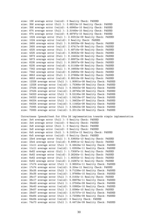
17](https://image.slidesharecdn.com/b1839bd1-2a78-4db3-9b3a-8259e67581a5-151102083036-lva1-app6892/85/bachelors_thesis_stephensen1987-17-320.jpg)
![Figure 2: Lena, the primary test image of use.
repetitions of that particular problem size.
All tests were done on an Intel Core 4x2 50Ghz i7-4710MQ. The testing goals are, and
will be tested, as follows:
• Correctness & error estimation: As mentioned previously, the error should be low.
Due to round-off errors, some error in the calculations is to be expected. An IEEE
754 double-precision floating point numbers has 52 bits for representing the fractional
part of the number. Since we get an extra bit of precision due to the first digit being
represented implicitly4, the error can thus at most be the difference in the last digits5
2−53 = 10−15.955. While it is theoretically possible to formally derive bounds on the
propagating error, the error is tightly connected to both the relative and absolute size
of the numbers. I therefore expect a result with too large an upper bound on the error
when compared to what is both acceptable and realistic. Previous work suggest the
error in general for different FFT methods increases as a factor of
√
N on average
where N is the input size [Duhamel and Vetterli, 1990]. Thus we should expect and
error of about
10−15.955
·
√
20402 ≈ 10−13
,
on average for the biggest input being transformed. Since every output value from the
convolution has passed two transforms, the error as a result of the convolution should
be around 10−10. As well as the average error, the maximum error is observed. This
is primarily to ensure no single significant error is hiding under a low average error.
These could come from boundary case errors for instance.
Using constructed M ×N input data such that the value at index (i, j) is i+j, and using
a 3 × 3 kernel with center (1, 1) and values 1/4 at indices {(0, 1), (1, 0), (2, 1), (1, 2)}
while leaving the rest zero, should return the input data as output in the valid region.
The upper edge (j = 0) should, except for corner pieces, have the convolved value
4
The fractional number is represented in a such way that the first bit is always one, and can therefore be
represented implicitly.
5
This is actually only true under the assumption that the exponent is 1.
18](https://image.slidesharecdn.com/b1839bd1-2a78-4db3-9b3a-8259e67581a5-151102083036-lva1-app6892/85/bachelors_thesis_stephensen1987-18-320.jpg)


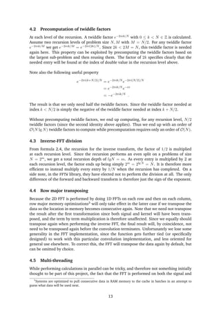
![7.5.4 Switching mechanism
Firstly, the switching mechanism seems to work. Secondly, considering that the input varies
quite a bit, and since hitting the exact crossover point between methods is practically impos-
sible due to random variations in the execution time. An error of less than 5% of the tested
input is quite respectable. That said, it’s hard to argue what is good. The particular input
sizes where the method has a tendency to choose the wrong method may be input sizes that
are used often in practice, or may not be used at all. It is most likely that the error happens
in areas where theres a crossover point. This could explain the grouping we see. In that
case, the difference in time used by either of the methods shouldn’t be too big, and choosing
the wrong method at these points is therefore of less concern as well.
7.5.5 Possible improvements
As noted already, complex multiplications with +1, −1, +i, −i can be regarded as free, and
since I did not exploit this, this is a simple way to reduce execution time. Using only features
from C, and thus skipping the overhead that comes along with C++ should, in the case of an
algorithm like this, yield substantially better results. If we instead wanted to save the mem-
ory use, one way is to only allocate space for the complex numbers, and then use the given
array for the real part of the number, thus getting closer to in-place calculations, but since
the two arrays is now not placed efficiently in memory, this is expected to slow computations
greatly. Alternatively, one could make assumptions on the input data, and assume the data
is already stored in an efficient complex data structure. However, this would violate a goal
in this project, to write a general-purpose implementation, and for that reason fit less in the
context of the SHARK library. I would therefore advice against any of these solutions.
When it comes to the FFTW library, its adaptive nature should resist most attempts to per-
form FFT faster using only a single FFT algorithm. If instead we went for a more realistic
goal just to have an implementation comparable to FFTW and Matlab, I would argue the di-
rection to take would be first to rewrite the code in a low level language such as C. Look
into ensuring memory allocation is efficient and thereafter take a look into implementing the
optimization I have done so far, and adjust it further by previously mentioned optimizations
while looking into even more ways to reduce the number of simple operations. Perhaps
even implementing the split-radix algorithm with the savings in operations count that fol-
lows along, and a mixed-radix implementation would remove most needs for zero-padding.
Doing small optimizations can seem like beating a dead horse, but as noted in [Frigo and
Johnson, 1998], FFT implementations consist of a large number of the same small opera-
tions, meaning a small increases in efficiency on these small operations often leads to great
gain in performance for the entire implementation. And in that regard, the Cooley-Tukey
Radix-2 implementation in this project may in fact be nearly comparable to other implemen-
tations.
8 Conclusions and Outlook
In this BSc thesis, I have shown how the Discrete Fourier Transform, through the convolu-
tion theorem, presents us with an indirect way to perform the convolution operation. I have
shown how it allows for reductions in computational complexity due to FFT algorithms re-
ducing the computational complexity to an order of O(n lg n) as opposed to the polynomial
O(n2).
During the project, an implementation of an indirect convolution method using the Cooley-
Tukey Radix-2 algorithm has been implemented with varying success. I conclude that the
27](https://image.slidesharecdn.com/b1839bd1-2a78-4db3-9b3a-8259e67581a5-151102083036-lva1-app6892/85/bachelors_thesis_stephensen1987-27-320.jpg)