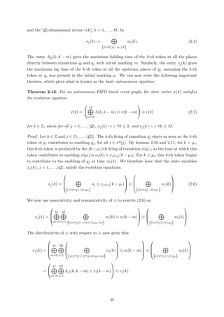
The document discusses max-plus algebra, which is the set Rmax = R ∪ {-∞} endowed with operations a ⊕ b = max{a,b} and a ⊗ b = a + b. It is shown that Rmax forms a semiring with additional useful properties. Chapter 1 introduces max-plus linear algebra concepts like vectors, matrices, eigenvalues/eigenvectors, and periodic behavior. Chapter 2 uses max-plus algebra to model discrete event systems and derive equations governing their time evolution. Chapter 3 extends this to stochastic event graphs and examines asymptotic firing rates and queuing system stability.
![Chapter 0
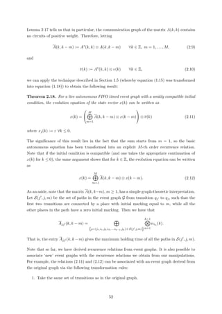
Introduction
Exotic semirings such as (R ∪ {−∞}, max, +) and (R ∪ {+∞}, min, +) have been studied at
length since the 1950s, beginning primarily in the area of operational research. Nowadays the
term ‘tropical mathematics’ is often used to describe their study, though this term originally
referred to one particular discrete version of the max-plus algebra introduced by I. Simon
in 1988 [15]. Their applications span a wide range of fields including optimisation & control,
mathematical physics, algebraic geometry, dynamic programming and mathematical biology [10,
15]. In particular, the study of such algebras in relation to discrete event system theory (both
deterministic and stochastic), graph theory, Markov decision processes, asymptotic analysis and
language theory has lead to some significant progress in these areas over the last 30 years [8].
Many of the concepts developed in conventional linear algebra have been ‘translated’ into the
world of max-plus, including solutions to linear and non-linear systems (both analytical and
numerical), linear dependence and independence, determinants, eigenvalues and eigenvectors
[9]. In 1979 Cuninghame-Green authored the first comprehensive unified account of these results
entitled “Minimax Algebra” [7], building on many papers published over the preceding 20 years
from various disciplines within mathematics, economics and computer science. As recently
as 2006, Heidergott, Olsder and Woude published what they consider the first ‘textbook’ in
the area of max-plus algebra [13], and many of the ideas explored below can be found in this
publication.
In the first chapter of this thesis, we aim to give an overview of max-plus linear algebra and
to build the necessary groundwork required for the applications discussed in the chapters that
follow. In particular, we present two celebrated theorems in the area of max-plus theory. The
first, which can be found in [7], concerns spectral theory and says that under mild conditions,
a matrix over the max-plus algebra has a unique eigenvalue with a simple graph-theoretic
interpretation. The second, originally proved by M. Viot in 1983 [2, 6], relates to the asymptotic
behaviour of sequential powers of max-plus matrices, which turns out to be essentially periodic
and has great implications for the material explored in Chapters 2 & 3.
In chapter 2 we introduce the concept of timed Petri nets & event graphs. For a thorough
1](https://image.slidesharecdn.com/10d08b3f-967c-4123-bade-f0ef8267a94d-151012204735-lva1-app6891/85/Thesis_JR-6-320.jpg)
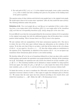
![discussion on the scope of their application readers are referred to [18]; in this thesis we fo-
cus solely on their use in the modelling of the time behaviour of a class of dynamic systems
known as ‘discrete event dynamic systems’. In simple terms, these are systems in which a finite
number of resources (e.g. processors or machines) are shared by several users (e.g. packets or
manufactured objects) which all contribute to the achievement of some common goal (e.g. a
parallel computation or the assembly of a product) [2]. We will see that under certain conditions
these systems, while highly non-linear in the conventional sense, can be ‘linearised’ by using
the max-plus algebra. This observation, first made in [5], is of vital importance and constitutes
one of the main reasons for the continued study of max-plus algebra today. The main content
of Chapter 2 concerns the ‘basic autonomous equation’ which governs the time evolution of
discrete event systems, and the steps towards its solution. We are then able to apply some ideas
from Chapter 1 to explore the long-term behaviour of such systems.
Chapter 3 concerns stochastic event graphs, which can be thought of as a natural extension
to the concepts introduced in Chapter 2. As the name suggests, we now assume a degree of
randomness in the event timings of the systems we are trying to model. Amongst other things,
stochastic event graphs can be used to model many types of queuing systems [3], the most
simple of which being the G/G/1 queue. We introduce several key ‘first order’ theorems which
establish the nature of stationary regimes in terms of the inverse throughput, and explore the
conditions under which such regimes are reached. We end by presenting a ‘second order’ theorem
concerning the stability of inter-event timings (for example, waiting times) in the context of
queuing systems.
2](https://image.slidesharecdn.com/10d08b3f-967c-4123-bade-f0ef8267a94d-151012204735-lva1-app6891/85/Thesis_JR-7-320.jpg)
![(a) εR × a = a × εR = εR
Note that the final axiom is not required in the definition of a standard ring since it follows
from the others, but it is needed here.
As the title of this section suggests, the max-plus algebra is a semiring with additive identity
ε := −∞ and multiplicative identity e := 0. It is straightforward to verify that all the axioms
of Definition 1.1 hold in the case of (Rmax, ⊕, ⊗). For example, the first distributive law holds
since
a ⊗ (b ⊕ c) = a + max{b, c}
= max{a + b, a + c}
= (a ⊗ b) ⊕ (a ⊗ c)
and the others follow similarly. For the sake of simplicity we will write Rmax for (Rmax, ⊕, ⊗)
when the context is clear.
Below we list three additional algebraic properties of Rmax which do not form part of the
definition of a semiring:
(i) Commutativity of ⊗:
∀a, b ∈ Rmax : a ⊗ b = b ⊗ a
(ii) Existence of multiplicative inverses:
∀a ∈ Rmax{ε} ∃ b ∈ Rmax such that a ⊗ b = e
(iii) Idempotency of ⊕:
∀a ∈ Rmax : a ⊕ a = a
The first two properties follow directly from the fact that (R, +) forms an abelian group, and
the third property is easily proved: a ⊕ a = max{a, a} = a. Properties (i) and (ii) mean that
we could refer to (Rmax, ⊕, ⊗) as a semifield (i.e. a field without additive inverses), though
this term can be ambiguous and is seldom used in mathematical literature. Note also that in
general, any semiring in which addition is idempotent we call an idempotent semiring. The term
dioid (originating from the phrase double monoid) was introduced by Baccelli et al. in 1992 to
mean idempotent semiring [2], but we do not use this word here.
The crucial difference between a semiring and a ring in general is that an element of the former
need not have an additive inverse. Note that this does not say that additive inverses can never
exist - there may be a non-empty subset of R containing elements which do have additive
inverses (which could be thought of as the additive analogue to the set of units in a standard
ring). However, the following lemma immediately tells us that no elements of Rmax (apart from
4](https://image.slidesharecdn.com/10d08b3f-967c-4123-bade-f0ef8267a94d-151012204735-lva1-app6891/85/Thesis_JR-9-320.jpg)
![way:
a⊗ n
m :=
n
m
× a
which is well-defined, assuming m = ε.
Next, we can equip the max-plus algebra with a natural order relation as follows:
Definition 1.3. For a, b ∈ Rmax, we say a ≤ b if a ⊕ b = b.
It is easily verified that the max-plus operations ⊕ and ⊗ preserve this order, i.e. ∀a, b, c ∈ Rmax,
a ≤ b ⇒ a ⊕ c ≤ b ⊕ c and a ⊗ c ≤ b ⊗ c.
Finally, infinite sums in max-plus are defined by i∈I xi := sup{xi : i ∈ I} for any possibly
infinite (even uncountable) family {xi}i∈I of elements of Rmax, when the supremum exists. In
general, we say that an idempotent semiring is complete if any such family has a supremum,
and if the product distributes over infinite sums. The max-plus semiring Rmax is not complete
(a complete idempotent semiring must have a maximal element), but it can be embedded in
the complete semiring (Rmax, ⊕, ⊗), where Rmax := Rmax ∪ {+∞}.
1.2 Vectors and Matrices over Rmax
1.2.1 Definitions and Structure
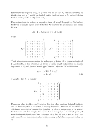
Let n, m ∈ N. We denote the set of n × m matrices over Rmax by Rn×m
max . For i ∈ {1, . . . , n},
j ∈ {1, . . . , m}, the element of a matrix A ∈ Rn×m
max in row i and column j is denoted by [A]ij,
or simply aij for notational convenience. Thus A ∈ Rn×m
max can be written as
a11 a12 · · · a1m
a21 a22 · · · a2m
...
...
...
...
an1 an2 · · · anm
where a11, . . . , anm ∈ Rmax. In a similar vein, the elements of Rn
max := Rn×1
max are called max-plus
vectors, and we write the i-th element of a vector x ∈ Rn
max as [x]i, or simply xi.
Typical concepts and operations from conventional algebra are defined for max-plus matrices
in the usual way (replacing + and × with ⊕ and ⊗ respectively), as outlined in the following
definitions.
Definition 1.4. The n × n max-plus identity matrix, denoted En, is defined by
[En]ij =
0 i = j
ε i = j
We will write E := En whenever the context is clear.
6](https://image.slidesharecdn.com/10d08b3f-967c-4123-bade-f0ef8267a94d-151012204735-lva1-app6891/85/Thesis_JR-11-320.jpg)
![Definitions 1.5. (i) For A, B ∈ Rn×m
max , their sum A ⊕ B is defined by
[A ⊕ B]ij = aij ⊕ bij = max aij, bij
(ii) For A ∈ Rn×k
max and B ∈ Rk×m
max , their product A ⊗ B is defined by
[A ⊗ B]il =
k
j=1
(aij ⊗ bjl) = max
j=1,...,k
(aij + bjl)
(iii) The transpose of a matrix A ∈ Rn×m
max is denoted by A and is defined as usual by
[A ]ij = [A]ji
(iv) For A ∈ Rn×n
max and k ∈ N, the k-th power of A, denoted A⊗k, is defined by
A⊗k
= A ⊗ A ⊗ · · · ⊗ A
k times
For k = 0, A⊗0 := En.
(v) For A ∈ Rn×m
max and α ∈ Rmax, α ⊗ A is defined by
[α ⊗ A]ij = α ⊗ [A]ij
We now look at a crucial result concerning the algebraic structure of square matrices over Rmax.
Proposition 1.6. (Rn×n
max , ⊕, ⊗) is an idempotent semiring with multiplicative identity En.
Proof. The axioms of Definition 1.1 all follow from the semiring structure of Rmax, and are
readily verified. For example, for A, B, C ∈ Rn×n
max we have that
[A ⊗ (B ⊕ C)]il =
n
j=1
(aij ⊗ (bjl ⊕ cjl))
=
n
j=1
(aij ⊗ bjl) ⊕ (aij ⊗ cjl)
=
n
j=1
(aij ⊗ bjl) ⊕
n
j=1
(aij ⊗ cjl)
= [(A ⊗ B) ⊕ (A ⊗ C)]il
and so A ⊗ (B ⊕ C) = (A ⊗ B) ⊕ (A ⊗ C). The other axioms follow similarly.
Note that since addition in (Rn×n
max , ⊕, ⊗) is idempotent, we can apply Lemma 1.2 once again to
see that no element of Rn×n
max has an additive inverse. However, unlike in Rmax, multiplication
7](https://image.slidesharecdn.com/10d08b3f-967c-4123-bade-f0ef8267a94d-151012204735-lva1-app6891/85/Thesis_JR-12-320.jpg)
![of matrices over Rmax is not commutative. For example
1 e
ε −2
2 −1
3 ε
=
3 e
1 ε
=
3 2
4 3
=
2 −1
3 ε
1 e
ε −2
Also unlike Rmax, matrices over Rmax do not necessarily have multiplicative inverses (i.e. they
are not necessarily invertible). We explore this in the next section.
1.2.2 Matrix Inversion
Definition 1.7. Let A, B ∈ Rn×n
max . B is a right inverse of A if A ⊗ B = E, and B is a left
inverse of A if B ⊗ A = E.
Definition 1.8. A max-plus permutation matrix is a matrix A ∈ Rn×n
max with each row and
each column containing exactly one entry equal to e, with all other entries equal to ε. If σ :
{1, . . . , n} → {1, . . . , n} is a permutation, the max plus permutation matrix Pσ is defined by
[Pσ]ij :=
e i = σ(j)
ε i = σ(j)
As the name suggests, left multiplication by Pσ permutes the rows of a matrix: the i-th row of
a matrix A ∈ Rn×n
max will appear as the σ(i)-th row of Pσ ⊗ A. For example, if n = 2 and σ is
defined by σ(1) = 2, σ(2) = 1:
ε e
e ε
1 2
3 4
=
3 4
1 2
Similarly, it is straightforward to see that right multiplication by Pσ permutes the columns of
a matrix.
Definition 1.9. A matrix A ∈ Rn×n
max is diagonal if [A]ij = ε for all i = j. If a1, . . . , an ∈
Rmax{ε}, the diagonal matrix D(a1, . . . , an) is defined by
[D(a1, . . . , an)]ij :=
ai i = j
ε i = j
Combining these two definitions, if σ is a permutation and a1, . . . , an ∈ Rmax {ε}, Pσ ⊗
D(a1, . . . , an) gives a matrix in which each row and each column contains exactly one finite
entry. This class of matrices (sometimes referred to as generalised permutation matrices) in
max-plus turns out to be of some significance, as the theorem below shows.
Theorem 1.10. A matrix A ∈ Rn×n
max has a right inverse if and only if A = Pσ ⊗ D(a1, . . . , an)
for some permutation σ and a1, . . . , an ∈ Rmax{ε}.
Proof. Suppose A = Pσ ⊗ D(a1, . . . , an) for some permutation σ and a1, . . . , an ∈ Rmax{ε}.
8](https://image.slidesharecdn.com/10d08b3f-967c-4123-bade-f0ef8267a94d-151012204735-lva1-app6891/85/Thesis_JR-13-320.jpg)
![Recalling from Section 1.1.1 that multiplicative inverses exist in Rmax, define B ∈ Rn×n
max by
[B]ij =
[A]⊗−1
ji if [A]ji = ε
ε otherwise
Then for i, j = 1, . . . , n we have that
[A ⊗ B]ij = max
k=1,...,n
aik ⊗ bkj
=
e j = i
ε j = i
Since if j = i, at least one of aik, bkj is equal to ε for each k = 1, . . . , n (since A only has one
finite element per column and row). Thus A ⊗ B = E, and B is a right inverse of A.
Conversely, suppose A has inverse B ∈ Rn×n
max . For i, j = 1, . . . , n we have
n
k=1
[A]ik ⊗ [B]kj = [E]ij
and therefore for each i = 1, . . . , n there is a (least) index c(i) (1 ≤ c(i) ≤ n) such that [A]ic(i)
and [B]c(i)i are both finite, since [E]ii = e. Moreover we cannot have [A]hc(i) finite with h = i,
since then
[A ⊗ B]hi ≥ [A]hc(i) ⊗ [B]c(i)i > ε = [E]hi
which contradicts our assumption that B is a right inverse of A. It follows that the mapping i →
c(i) is a bijection, i.e. each column of A is labelled c(i) for some i and contains exactly one finite
element, and each row of A contains exactly one finite element. That is, A = Pσ ⊗D(a1, . . . , an)
for some permutation σ and a1, . . . , an ∈ Rmax{ε}.
Theorem 1.11. For A, B ∈ Rn×n
max , A ⊗ B = E if and only if B ⊗ A = E (i.e. right and left
inverses are equivalent), and A uniquely determines B.
Proof. Suppose that A has right inverse BR ∈ Rn×n
max . Then by Theorem 1.10, we know that
A = Pσ ⊗ D(a1, . . . , an) for some permutation σ and a1, . . . , an ∈ Rmax{ε}. Now, as before,
define BL ∈ Rn×n
max by
[BL]ij =
[A]⊗−1
ji if [A]ji = ε
ε otherwise
and using the same reasoning as before we observe that BL is a left inverse of A. Finally, note
that
BR = E ⊗ BR = (BL ∗ A) ⊗ BR = BL ⊗ (A ⊗ BR) = BL ⊗ E = BL
showing that BR is uniquely determined, and is also a left inverse.
9](https://image.slidesharecdn.com/10d08b3f-967c-4123-bade-f0ef8267a94d-151012204735-lva1-app6891/85/Thesis_JR-14-320.jpg)
![Note that, crudely put, the permanent is the max-plus analogue of the determinant with the
minuses simply removed. We can understand the formula to give the maximal sum of the
diagonal values for all permutations of the columns of A. The permanent has been studied at
length both in the case of conventional algebra (see [17]) and in max-plus & related semirings
(see [19]).
Note that if A ∈ Rn×n
max is invertible then by Theorem 1.10, A = Pσ ⊗ D(a1, . . . , an) and so
perm(A) = n
i=1 ai = ε. However, unlike in the case of determinants in conventional matrix
algebra, the converse is not necessarily true.
The second concept in max-plus related to the determinant, known as the dominant, can be
thought of as a refinement of the permanent. It is defined below.
Definition 1.14. Let A ∈ Rn×n
max and let the matrix zA be defined by [zA]ij = zaij . The dominant
of A, denoted dom(A), is defined as
dom(A) =
highest exponent in det(zA) if det(zA) = 0
ε otherwise
The dominant can be used to prove max-plus analogues of major results such as Cramér’s
Theorem and the Cayley-Hamilton Theorem. We do not have the space to include these here;
for a comprehensive discussion readers are again referred to [19].
1.3 Graph-theoretic Interpretations in Max-Plus
As in conventional linear algebra, when working with vectors and matrices it is often natural
to interpret definitions and theorems graphically. It turns out that in the case of max-plus
algebra, it is not only natural to do so but also rather insightful. We will only really be able to
appreciate this when we come to look at the eigenvalue problem in the next section, but firstly
we must define all of the graph-theoretic concepts that we will require.
Definitions 1.15. (i) A directed graph G is a pair (V, E) where V is the set of vertices (or
nodes) and E ⊆ V × V is the set of edges (or arcs).
(ii) A path from vertex i to vertex j is a sequence of edges p = (i1, . . . , is+1) with i1 = i and
is+1 = j, such that (ik, ik+1) ∈ E for all k ∈ {1, . . . , s}.
(iii) The length of a path p = (i1, . . . , is+1), denoted |p|l, is equal to s. The set of paths from
vertex i to vertex j of length k is denoted Pk(i, j).
(iv) The weight of a path p from vertex i to vertex j of length d is given by
|p|w =
d
k=1
aik+1,ik
where i1 = i and id+1 = j.
11](https://image.slidesharecdn.com/10d08b3f-967c-4123-bade-f0ef8267a94d-151012204735-lva1-app6891/85/Thesis_JR-16-320.jpg)
![(v) The average weight of a path p is given by |p|w
|p|l
.
(vi) A circuit of length s is a path of length s which starts and finishes at the same vertex, i.e.
a path c = (i1, . . . , is+1) such that i1 = is+1.
(vii) A circuit c = (i1, . . . , is+1) is elementary if i1, . . . , is are distinct, and s ≥ 1. We denote
the set of elementary circuits in G(A) by C(A).
(viii) For A ∈ Rn×n
max , the communication graph (or the precedence graph) of A, denoted G(A),
is the graph with vertex set V(A) = {1, . . . , n} and edge set E(A) = {(i, j) : aji = ε}. The
weight of the edge (i, j) ∈ E(A) is given by the entry aji.
Note that the (i, j)-th entry of the matrix A specifies the weight of the edge in G(A) from vertex
j to vertex i. This is common practice in the area of max-plus and graph theory but may not
appear intuitive to those new to the subject.
We now move on to looking at two particular matrices that play a vital role in relating graph
theory to max-plus linear algebra. For A ∈ Rn×n
max , let
A+
:=
∞
k=1
A⊗k
The element [A+]ji gives the maximal weight of any path from i to j in G(A). This statement
is non-trivial, but follows directly from the theorem below.
Theorem 1.16. Let A ∈ Rn×n
max . Then ∀k ∈ N:
[A⊗k
]ji =
max |p|w : p ∈ Pk(i, j) if Pk(i, j) = ∅
ε if Pk(i, j) = ∅
Proof. We use induction on k. Let i, j ∈ {1, . . . , n}. When k = 1, P1(i, j) either contains a
single path of length 1, namely the edge (i, j), or is empty if no such edge exists. In the first case,
the weight of the path is by definition [A]ji, and in the second case max |p|w : p ∈ Pk(i, j) = ε,
which is again equal to the value [A]ji (since there is no edge from i to j).
Now suppose the result holds for some k. Firstly, assume that Pk+1(i, j) = ∅. A path p ∈
Pk+1(i, j) can be split up into a subpath of length k running from i to some vertex l, and a
path consisting of a single edge from l to j. More formally:
p = ˆp ◦ (l, j) with ˆp ∈ Pk(i, l)
The maximal weight of any path in Pk+1(i, j) can thus be obtained from
max
l=1,...,n
[A]jl + max{|ˆp|w : ˆp ∈ Pk(i, l)}
= max
l=1,...,n
[A]jl + [A⊗k
]li (Inductive hypothesis)
12](https://image.slidesharecdn.com/10d08b3f-967c-4123-bade-f0ef8267a94d-151012204735-lva1-app6891/85/Thesis_JR-17-320.jpg)
![=
n
l=1
[A]jl ⊗ [A⊗k
]li
= [A ⊗ A⊗k
]ji
= [A⊗(k+1)
]ji
which is what we wanted to prove. Finally, consider the case when Pk+1(i, j) = ∅; i.e. when
there exists no path of length k + 1 from i to j. This implies that for any vertex l, either there
is no path of length k from i to l or there is no edge from l to j (or possibly both). Hence
for any l, at least one of the values [A]jl, [A⊗k]li equals ε. Therefore [A⊗(k+1)]ji = ε, and this
completes the proof.
Note that Theorem 1.16 immediately tells us that A+ is not necessarily well-defined. For
example, if there exists a circuit c = (i1, . . . , is+1) in G(A) in which every edge has positive
weight, then [A⊗k]ji diverges (i.e. tends to +∞) as k → ∞ for any i, j ∈ {i1, . . . , is+1} (since
we can loop around the circuit c as many times a we like, creating a path of higher and higher
weight). The next lemma provides us with a sufficient condition for A+ to be well-defined, and
also reduces the complexity of the infinite sum.
Lemma 1.17. Let A ∈ Rn×n
max be such that any circuit in G(A) has non-positive average weight
(i.e. less than or equal to e). Then we have
A+
= A⊗1
⊕ A⊗2
⊕ A⊗3
⊕ · · · ⊕ A⊗n
∈ Rn×n
max
Proof. Since A is of dimension n, any path p in G(A) from i to j of length greater than n
necessarily contains at least one circuit. We have assumed that all of the circuits in G(A) have
non-positive weights, so removing the circuits in p yields a path from i to j of length at most
n, and of greater average weight. It follows that
[A+
]ji ≤ max [A⊗k
]ji : k ∈ {0, . . . , n}
and the reverse inequality is immediate from the definition of A+. This concludes the proof.
Before moving on, we prove one simple property of A+ that will come in handy later on.
Proposition 1.18. For A ∈ Rn×n
max , we have that A+ ⊗ A+ = A+.
Proof. Consider two vertices i, l ∈ {1, . . . , n}. A path of maximal weight from i to l can be split
up as a path of maximal weight from i to j plus a path of maximal weight from j to l, for any
j ∈ {1, . . . , n} for which the sum of the two path weights is maximal. Indeed this relationship
holds if and only if j is in the path of maximal weight from i to l, but for our purposes we can
simply take the maximum over all vertices.
By Theorem 1.16, the weight of such a path is given by [A+]li. Thus in max-plus notation
13](https://image.slidesharecdn.com/10d08b3f-967c-4123-bade-f0ef8267a94d-151012204735-lva1-app6891/85/Thesis_JR-18-320.jpg)
![(recalling that ⊗ is commutative for scalars α ∈ Rmax), we can write
[A+
]li =
n
j=1
[A+
]ji ⊗ [A+
]lj
=
n
j=1
[A+
]lj ⊗ [A+
]ji = [A+
⊗ A+
]li
and therefore A+ = A+ ⊗ A+ as required.
We now introduce one more definition which is closely related to the object A+ defined above.
This will prove to be an integral concept throughout the rest of this chapter and beyond, and
as such, this is one of the most important definitions in this thesis.
Definition 1.19. For A ∈ Rn×n
max , let
A∗
:=
∞
k=0
A⊗k
= E ⊕ A+
Clearly, A∗ and A+ only differ on the leading diagonal. By Theorem 1.16, the (j, i)-th of A∗
could be interpreted as the maximal weight of any path from i to j in G(A), provided we
recognise the additional concept of an empty circuit of length 0 and weight e from every vertex
to itself.
Using Lemma 1.17, it is immediate from the definition of A∗ that if all the circuits in G(A) have
non-positive average weight, then A∗ = A⊗0 ⊕ A⊗1 ⊕ · · · ⊕ A⊗n. However, as the lemma below
shows, thanks to the addition of the identity matrix (i.e. the A⊗0 term) in A∗, we are able to
refine this result slightly by dropping the final term in the sum.
Lemma 1.20. Let A ∈ Rn×n
max be such that any circuit in G(A) has non-positive average weight.
Then we have
A∗
= A⊗0
⊕ A⊗1
⊕ A⊗2
⊕ · · · ⊕ A⊗(n−1)
∈ Rn×n
max
Proof. The same argument applies as in the proof of Lemma 1.17. Note that any path p in G(A)
from i to j of length n or greater necessarily contains at least one circuit, and so removing the
circuit(s) yields a path from i to j of length at most n − 1 and with greater average weight. For
the special case when i = j and p is an elementary circuit of length n (so visiting each vertex
in G(A) exactly once), the i-th entry on the diagonal of A⊗0 (which equals e by definition) will
always be greater than the corresponding entry in A⊗n, since e is the maximum possible weight
of any circuit. This is why we can drop the A⊗n term.
Note that we also have a direct analogue of Lemma 1.18 for the matrix A∗, and this will be
useful in the analysis that follows:
Proposition 1.21. For A ∈ Rn×n
max , we have that A∗ ⊗ A∗ = A∗.
14](https://image.slidesharecdn.com/10d08b3f-967c-4123-bade-f0ef8267a94d-151012204735-lva1-app6891/85/Thesis_JR-19-320.jpg)
![Proof. From Lemma 1.18 we have that A+ = A+ ⊗A+. Recalling the definition of A∗ and using
idempotency of matrix addition, we have
A∗
⊗ A∗
= (A+
⊕ E) ⊗ (A+
⊕ E)
= (A+
⊗ A+
) ⊕ (A+
⊗ E) ⊕ (E ⊗ A+
) ⊕ E
= A+
⊕ A+
⊕ A+
⊕ E
= A+
⊕ E = A∗
as required.
To finish this section, we introduce one more important property of square matrices over max-
plus known as irreducibility. The definition comes in three parts:
Definitions 1.22. (i) In a graph G, a vertex j is reachable from vertex i if there exists a
path from i to j.
(ii) A graph is strongly connected if every vertex is reachable from every other vertex.
(iii) A matrix A ∈ Rn×n
max is irreducible if G(A) is strongly connected.
The class of irreducible matrices over max-plus will turn out to be of real significance in Section
1.4. From a practical point of view it is not obvious how to determine whether a given matrix
A ∈ Rn×n
max is irreducible, but as the proposition below shows, one option is to examine the matrix
A+. Combined with Lemma 1.17 (when A has the appropriate properties), this provides us with
a handy (and computationally quick) way to check for matrix irreducibility over max-plus.
Proposition 1.23. A matrix A ∈ Rn×n
max is irreducible if and only if all the entries of A+ are
different from ε.
Proof. A matrix is irreducible if there is a path between any two vertices i and j in G(A), which
by Theorem 1.16 occurs exactly when the entry [A+]ji is not equal to ε.
1.4 Spectral Theory
1.4.1 Eigenvalues and Eigenvectors
Given a matrix A ∈ Rn×n
max , we consider the problem of existence of eigenvalues and eigenvectors.
The main result in max-plus spectral theory is that, under mild conditions, A has a unique
eigenvalue with a simple graph-theoretic interpretation. As can be seen below, the definition of
max-plus eigenvalues and eigenvectors is a direct translation from conventional linear algebra,
with the × operator replaced with ⊗:
Definition 1.24. Let A ∈ Rn×n
max . If there exists a scalar µ ∈ Rmax and a vector v ∈ Rn
max
(containing at least one finite element) such that
A ⊗ v = µ ⊗ v
15](https://image.slidesharecdn.com/10d08b3f-967c-4123-bade-f0ef8267a94d-151012204735-lva1-app6891/85/Thesis_JR-20-320.jpg)
![then µ is an eigenvalue of A and v is an eigenvector of A associated with the eigenvalue µ.
Note that Definition 1.24 allows an eigenvalue to be µ = ε. However, the proposition below says
that this can only happen when A has a column in which all entries are ε. In graph-theoretic
terms this means that G(A) has a vertex which, once visited, can never be left (sometimes called
a sink). This is uninteresting from an analytical point of view, so it is reasonable to consider
the case µ = ε to be trivial. Before we prove this result, we introduce some simple notation.
Notation. Let A ∈ Rn×n
max . For i ∈ {1, . . . , n}, we denote the i-th row of A by [A]i·. Similarly,
for j ∈ {1, . . . , n}, we denote the j-th column of A by [A]·j.
Proposition 1.25. ε is an eigenvalue of A ∈ Rn×n
max iff A has at least one column in which all
entries are ε.
Proof. Let A ∈ Rn×n
max be such that [A]·j = (ε, . . . , ε) for some j ∈ {1, . . . , n}. Let v ∈ Rn
max be
such that [v]i = ε ∀i = j and [v]j = α = ε. Then it is easy to verify that [A ⊗ v]i = ε for all
i = 1, . . . , n; that is, ε is an eigenvalue of A with an associated eigenvector v.
Conversely, suppose A ∈ Rn×n
max has eigenvalue ε with an associated eigenvector v. let J = {j :
vj = ε}, which is non-empty by definition. Then for each i = 1, . . . , n we have
ε = [A ⊗ v]i =
n
j=1
aij ⊗ vj =
j∈J
aij ⊗ vj
=⇒ aij = ε ∀j ∈ J
So every column j of A for which vj = ε has all its entries equal to ε. In particular, A contains
at least one column in which all entries are ε.
Corollary 1.26. If A ∈ Rn×n
max is irreducible then ε is not an eigenvalue of A.
Proof. If A is irreducible then it cannot have a column in which all entries are ε. Thus by
Proposition 1.25, ε is not an eigenvalue of A.
Note that eigenvectors are not unique: any scalar multiple of an eigenvector is also an eigen-
vector, and more generally, if µ is an eigenvalue of A, v1, v2 are associated eigenvectors and
α1, α2 ∈ Rmax{ε}, then we have
A ⊗ (α1 ⊗ v1) ⊕ (α2 ⊗ v2) = A ⊗ (α1 ⊗ v1) ⊕ A ⊗ (α2 ⊗ v2)
= α1 ⊗ (A ⊗ v1) ⊕ α2 ⊗ (A ⊗ v2)
= α1 ⊗ (µ ⊗ v1) ⊕ α2 ⊗ (µ ⊗ v2)
= µ ⊗ (α1 ⊗ v1) ⊕ (α2 ⊗ v2)
So (α1 ⊗ v1) ⊕ (α2 ⊗ v2) is also an eigenvector associated with the eigenvalue µ. In fact, the
eigenvectors associated with a given eigenvalue form a vector space in max-plus called the
eigenspace which we shall explore in depth later.
16](https://image.slidesharecdn.com/10d08b3f-967c-4123-bade-f0ef8267a94d-151012204735-lva1-app6891/85/Thesis_JR-21-320.jpg)
![As we mentioned at the beginning of Section 1.3, many of the results in the area of max-plus
spectral theory can be interpreted graphically, and the next key lemma constitutes the first step
in doing just that.
Lemma 1.27. Let A ∈ Rn×n
max have finite eigenvalue µ. Then µ is the average weight of some
elementary circuit in G(A).
Proof. Let v be an associated eigenvector of µ. Then by definition not all the entries of v equal
ε, i.e. there exists a vertex/index j1 ∈ {1, . . . , n} such that vj1 = ε. Now v is an eigenvector
and so we have [A ⊗ v]j1 = µ ⊗ vj1 = ε. But [A ⊗ v]j1 = n
k=1 aj1k ⊗ vk, and therefore there
exists a vertex j2 such that
aj1j2 ⊗ vj2 = [A ⊗ v]j1 = ε (1.1)
which implies aj1j2 = ε, i.e. (j2, j1) is an edge in G(A). (1.1) also implies that vj2 = ε, so we
can continue in the same fashion to find a vertex j3 with (j3, j2) an edge in G(A) and vj3 = ε.
Proceeding in this way, eventually some vertex, say, vertex jh, must be encountered for a second
time since the number of vertices is finite. Thus by ignoring the edges prior to encountering jh
for the first time, we have found an elementary circuit
c = ((jh, jh+l−1), (jh+l−1, jh+l−2), . . . , (jh+1, jh))
of length |c|l = l, and with weight
|c|w =
l−1
k=0
ajh+kjh+k+1
(1.2)
where jh = jh+l. By construction, we have that
l−1
k=0
(ajh+kjh+k+1
⊗ vjh+k+1
) = µ⊗l
⊗
l−1
k=0
vjh+k
or equivalently in conventional algebra (for ease of manipulation):
l−1
k=0
ajh+kjh+k+1
+ vjh+k+1
= (l × µ) +
l−1
k=0
vjh+k
Now, because jh = jh+l it follows that l−1
k=0 vjh+k+1
= l−1
k=0 vjh+k
, so subtracting l−1
k=0 vjh+k
from both sides yields
l−1
k=0
ajh+k
jh+k+1 = l × µ
and translated back into max-plus, we can substitute this into (1.2) to see that |c|w = µ⊗l.
17](https://image.slidesharecdn.com/10d08b3f-967c-4123-bade-f0ef8267a94d-151012204735-lva1-app6891/85/Thesis_JR-22-320.jpg)
![Thus we have that the average weight of the circuit c is equal to
|c|w
|c|l
=
µ⊗l
l
= µ
as required.
Lemma 1.27 tells us that the only candidates for eigenvalues are the average weights of circuits
in G(A). However, it does not tell us which circuits actually define an eigenvalue and which
do not. Fortunately, when A is irreducible the answer to this question is very simple: only
the maximal average circuit weight defines an eigenvalue. This result is established in the two
theorems below, but first we require some additional definitions and notation.
Definitions 1.28. (i) A circuit c ∈ C(A) is critical if its average weight is maximal.
(ii) For A ∈ Rn×n
max , the critical graph of A, denoted Gc(A), is the graph containing the vertices
and edges which belong to the critical circuits in G(A). We write Gc(A) = (Vc(A), Ec(A)),
and refer to the vertices in Vc(A) as critical vertices.
(iii) The critical classes of A ∈ Rn×n
max are the maximal strongly connected components of Gc(A).
Notation. Let A ∈ Rn×n
max . For β ∈ Rmax{ε}, define the matrix Aβ by [Aβ]ij = aij − β.
Note that the ‘−’ operator is to be interpreted in conventional algebra, where we adopt the
convention ε − x = ε ∀x ∈ R. If β is an eigenvalue of A, the matrix Aβ is sometimes called the
normalised matrix.
Note that the communication graphs G(A) and G(Aβ) are identical except for their edge weights,
and if a circuit c in G(A) has average weight w then the same circuit in G(Aβ) has average weight
w − β. In particular, if G(A) has finite maximal average circuit weight λ then the maximal
average circuit weight in G(Aλ) is λ − λ = 0. Furthermore, a circuit in G(A) is critical if and
only if it is critical in G(Aλ), and therefore Gc(A) and Gc(Aλ) are identical (again, except for
their edge weights).
Consider the matrix A+
λ , which is to be read (Aλ)+
. By Theorem 1.16, the element [A+
λ ]ij gives
the maximal weight of any path from j to i in G(Aλ). In particular, since all circuits in G(Aλ)
have non-positive average weight, we must have [A+
λ ]ii ≤ e for all i ∈ {1, . . . , n}. Furthermore,
for the matrix A∗
λ (also to be read (Aλ)∗
) we obtain [A∗
λ]ii = e⊕[A+
λ ]ii = e for all i ∈ {1, . . . , n}.
Theorem 1.29. Let the communication graph G(A) of a matrix A ∈ Rn×n
max have finite maximal
average circuit weight λ. Then λ is an eigenvalue of A, with an associated eigenvector [A∗
λ]·j
for any vertex j ∈ Vc(A).
Proof. Firstly note that all the circuits in G(Aλ) have non-positive average weight, and therefore
A+
λ is well-defined by Lemma 1.17. Now, every vertex in Gc(Aλ) is contained in a non-empty
circuit which has weight e, i.e.
∀j ∈ Vc
(A) : [A+
λ ]jj = e (1.3)
18](https://image.slidesharecdn.com/10d08b3f-967c-4123-bade-f0ef8267a94d-151012204735-lva1-app6891/85/Thesis_JR-23-320.jpg)
![Next, write
[A∗
λ]ij = [E ⊕ A+
λ ]ij =
ε ⊕ [A+
λ ]ij for i = j
e ⊕ [A+
λ ]ij for i = j
Then from (1.3), for j ∈ Vc(A) it follows that
[A+
λ ]·j = [A∗
λ]·j (1.4)
Now, note that we have
A+
λ = A⊗1
λ ⊕ A⊗2
λ ⊕ . . .
= Aλ ⊗ (A⊗0
λ ⊕ A⊗1
λ ⊕ . . . ) = Aλ ⊗ A∗
λ
So substituting this into (1.4) gives for j ∈ Vc(A)
[Aλ ⊗ A∗
λ]·j = [A∗
λ]·j ⇐⇒ Aλ ⊗ [A∗
λ]·j = [A∗
λ]·j
⇐⇒ A ⊗ [A∗
λ]·j = λ ⊗ [A∗
λ]·j
Therefore λ is an eigenvalue of A and the j-th column of A∗
λ is an associated eigenvector for
any j ∈ Vc(A).
Theorem 1.30. Let A ∈ Rn×n
max be irreducible. Then A has a unique eigenvalue, denoted λ(A),
which is finite and equal to the maximal average circuit weight in G(A).
Proof. Let the maximal average circuit weight in G(A) be denoted by λ. Since A is irreducible,
G(A) must contain a circuit and therefore λ is necessarily finite. Thus by Theorem 1.29 we
know that λ is an eigenvalue of A, and it remains to show uniqueness.
Let c = (j1, . . . , jl+1) be an arbitrary circuit in C(A) of length l = |c|l, with jl+1 = j1. Then
ajk+1jk
= ε for all k ∈ {1, . . . , l}. Further, suppose that µ is an eigenvalue of A with an associated
eigenvector v. Note that A is irreducible, so by Corollary 1.26 we have that µ = ε. Now, since
A ⊗ v = µ ⊗ v, it follows that
ajk+1jk
⊗ vjk
≤ µ ⊗ vjk+1
, k ∈ {1, . . . , l}.
and arguing as in Lemma 1.27 (replacing equalities with the appropriate inequalities), we see
that the average weight of the circuit c satisfies
|c|w
|c|l
≤
µ⊗l
l
= µ (1.5)
That is, µ ≥ λ (since (1.5) holds for all c ∈ C(A), and we already have that the maximal
average circuit weight is λ). But by Lemma 1.27, µ is equal to the average weight of some
circuit c ∈ C(A), and so µ ≤ λ also. Hence µ = λ, i.e. λ is the unique eigenvalue of A.
19](https://image.slidesharecdn.com/10d08b3f-967c-4123-bade-f0ef8267a94d-151012204735-lva1-app6891/85/Thesis_JR-24-320.jpg)
![When A is large it is often difficult to identify the maximal average circuit weight in G(A). In
fact, there exist several numerical procedures used to determine the eigenvalue of an irreducible
matrix in max-plus, including Karp’s Algorithm and the Power Algorithm. However, none of
these has a particularly attractive order of complexity - for example, the complexity of Karp’s
Algorithm is of order n3, and the complexity of the Power Algorithm is not known precisely
(see [11]). We do not have space here to describe the methods in detail; for more information
readers are referred to chapter five of [13].
We end this section with a simple proposition that, while interesting in its own right, will come
in handy when we begin to look at the eigenspace.
Proposition 1.31. Let A ∈ Rn×n
max be an irreducible matrix with eigenvalue λ and associated
eigenvector v. We have that vi > ε for all i ∈ {1, . . . , n}.
Proof. Call the set of vertices of G(A) corresponding to the finite entries of v the support of
v, denoted Z(v). Suppose that Z(v) does not contain all the elements of V(A). Since A is
irreducible, there must be edges from the vertices in Z(v) to vertices not belonging to Z(v).
Hence there exists vertices j ∈ Z(v), i /∈ Z(v) with aij = ε. Then
[A ⊗ v]i ≥ aij ⊗ vj > ε
That is, Z(A ⊗ v) is strictly bigger than Z(v). But A ⊗ v = λ ⊗ v (and λ is finite by Theorem
1.30), so Z(v) and Z(A⊗v) should be equal. This is a contradiction, and so Z(v) must contain
all the elements of V(A).
1.4.2 The Eigenspace
Let A ∈ Rn×n
max have finite eigenvalue λ. In this part of our analysis we let V (A, λ) denote the
set of all eigenvectors of A associated with the eigenvalue λ, which we call the eigenspace of A
w.r.t. λ. If A is irreducible then by Theorem 1.30 we know that it has a unique eigenvalue, so
we can drop the dependence on λ and denote the eigenspace of A simply by V (A).
The main aim of this section is to find an expression that completely characterises the eigenspace
of A. In Theorem 1.29 we established that [A∗
λ]·j is an eigenvector of A for any j ∈ Vc(A),
but are these the only eigenvectors (of course, up to taking linear combinations, as discussed
above)? We will eventually see that the answer to this question is yes, but first we require some
intermediate steps.
Lemma 1.32. Let A ∈ Rn×n
max . We have that A∗
λ = (E ⊕ Aλ)⊗(n−1).
Proof. If n = 1 then the result is trivial. Otherwise, since E and Aλ commute, we can carry
out the iterated multiplication (E ⊕ Aλ) ⊗ · · · ⊗ (E ⊕ Aλ) to obtain
(E ⊕ Aλ)⊗(n−1)
= E ⊕
n−1
i=1
A⊗i
λ ⊕ · · · ⊕ A⊗i
λ
(n−1
i ) times
(1.6)
20](https://image.slidesharecdn.com/10d08b3f-967c-4123-bade-f0ef8267a94d-151012204735-lva1-app6891/85/Thesis_JR-25-320.jpg)
![Each power A⊗0
λ , . . . , A
⊗(n−1)
λ occurs at least once, so by idempotency of ⊕, (1.6) becomes
(E + Aλ)⊗(n−1)
= E ⊕ Aλ ⊕ A⊗2
λ ⊕ . . . A
⊗(n−1)
λ (1.7)
However, noting that every circuit in G(Aλ) must have non-positive weight, we can apply Lemma
1.20 to see that the right-hand side of (1.7) is equal to A∗
λ. This completes the proof.
Lemma 1.33. Let A ∈ Rn×n
max be an irreducible matrix, with eigenvalue λ and an associated
eigenvector v. Then the matrix A∗
λ has eigenvalue e, also with an associated eigenvector v.
Proof. Firstly, note that for any j ∈ {1, . . . , n}
[λ ⊗ v]j = [A ⊗ v]j ⇐⇒ vj = [A ⊗ v]j − λ ⇐⇒ e ⊗ vj = [Aλ ⊗ v]j
That is, e ⊗ v = Aλ ⊗ v, and v is also an eigenvector of Aλ (whose unique eigenvalue must be e
by Theorem 1.30). Thus the eigenspaces V (A) and V (Aλ) coincide. Next, note that
(E ⊕ Aλ) ⊗ v = (E ⊗ v) ⊕ (Aλ ⊗ v) = v ⊕ v = v
Therefore, using Lemma 1.32:
A∗
λ ⊗ v = (E ⊕ Aλ)⊗(n−1)
⊗ v = v = e ⊗ v
as required.
Definition 1.34. Let A ∈ Rn×n
max be a matrix with eigenvalue λ and associated eigenvector v.
The saturation graph of A with respect to λ, denoted Sλ(A, v), is the graph consisting of those
edges (j, i) ∈ E(A) such that aij ⊗ vj = λ ⊗ vi, with vi, vj = ε.
Recall that by definition, if v is an eigenvector of A then there exists at least one i ∈ {1, . . . , n}
such that vi = ε. Then, since A ⊗ v = λ ⊗ v we have that n
j=1 aij ⊗ vj = λ ⊗ vi, which implies
that there exists (at least one) j ∈ {1, . . . , n} such that aij ⊗ vj = λ ⊗ vi. This value is finite
(assuming λ = ε), so we must have (j, i) ∈ E Sλ(A, v) . That is, the saturation graph of A
w.r.t. λ is never empty. Indeed, if A is irreducible, by Proposition 1.31 we know that vi > ε for
all i ∈ {1, . . . , n}, and so by the same argument, Sλ(A, v) contains all the vertices in V(A). In
this case we know that the eigenvalue λ is unique, and therefore we drop the dependence on λ
and simply refer to the saturation graph of A.
Lemma 1.35. Let A ∈ Rn×n
max be an irreducible matrix, with eigenvalue λ and associated eigen-
vector v. We have:
(i) For each vertex i ∈ V(A), there exists a circuit in S(A, v) from which vertex i can be
reached in a finite number of steps.
(ii) Any circuit in S(A, v) belongs to Gc(A).
Proof. (i) A is irreducible, so by Proposition 1.31 we know that vi > ε for all i ∈ {1, . . . , n}. Let
21](https://image.slidesharecdn.com/10d08b3f-967c-4123-bade-f0ef8267a94d-151012204735-lva1-app6891/85/Thesis_JR-26-320.jpg)
![i ∈ V(A), which by the discussion above we know is a vertex of the saturation graph S(A, v).
Thus there is a vertex j such that λ ⊗ vi = aij ⊗ vj. Repeating this argument, we can identify
a vertex k such that λ ⊗ vj = ajk ⊗ vk. Repeating this argument an arbitrary number of times,
say, m, we get a path in S(A, v) of length m. If m > n, the constructed path must contain a
circuit.
(ii) Let c = (i1, i2, . . . , il+1) be a circuit of length l in S(A, v). By definition, for all k ∈ {1, . . . , n}
we have that
λ ⊗ vik+1
= aik+1ik
⊗ vik
which implies that
λ⊗l
⊗ vi1 =
l
k=1
aik+1ik
⊗ vi1
Hence, recalling that vi1 is finite:
λ⊗l
=
l
k=1
aik+1ik
But the right-hand side is simply equal to the weight of the circuit c, which thus has average
weight λ. But A is irreducible, so by Theorem 1.30 λ is equal to the maximal average circuit
weight in G(A). Thus c is critical, and belongs to Gc(A).
Lemma 1.36. Let A ∈ Rn×n
max be an irreducible matrix, with eigenvalue λ and associated eigen-
vector v. Then v can be written as
v =
j∈Vc(A)
αj ⊗ [A∗
λ]·j
for some αj ∈ Rmax, j ∈ Vc(A).
Proof. Consider two vertices i, j in S(Aλ, v) such that there exists a path from i to j, say,
(i1, i2, . . . , il+1), with i1 = i and il+1 = j. Then by definition of the saturation graph, this gives
[Aλ]ik+1ik
⊗ vik
= vik+1
, k ∈ {1, . . . , l}
Hence vj = a ⊗ vi, where a is given by
a =
l
k=1
[Aλ]ik+1ik
≤ [A⊗l
λ ]ji ≤ [A∗
λ]ji (1.8)
Now, using that vj = a ⊗ vi, for an arbitrary vertex ν ∈ {1, . . . , n}:
[A∗
λ]νj ⊗ vj = [A∗
λ]νj ⊗ a ⊗ vi
≤ [A∗
λ]νj ⊗ [A∗
λ]ji ⊗ vi (by (1.8))
22](https://image.slidesharecdn.com/10d08b3f-967c-4123-bade-f0ef8267a94d-151012204735-lva1-app6891/85/Thesis_JR-27-320.jpg)
![≤ [A∗
λ]νi ⊗ vi (1.9)
where the last inequality follows from Proposition 1.21. By applying Lemma 1.35, for any vertex
j in S(Aλ, v) there exists a vertex i = i(j) ∈ Vc(A). Inequality (1.9) therefore implies
j∈S(Aλ,v)
[A∗
λ]νj ⊗ vj ≤
i∈Vc(Aλ)
[A∗
λ]νi ⊗ vi (1.10)
and this holds for any ν ∈ {1, . . . , n}.
Now, by Lemma 1.33, A∗
λ has eigenvalue e with an associated eigenvector v, i.e. v = A∗
λ ⊗ v.
The value of vν is equal to [A∗
λ]νj ⊗vj for some j, which by definition has to be in the saturation
graph S(Aλ, v). Thus it holds for ν ∈ {1, . . . , n} that
vν =
j∈S(Aλ,v)
[A∗
λ]νj ⊗ vj
(1.10)
≤
j∈Vc(Aλ)
[A∗
λ]νj ⊗ vj
On the other hand, since v is an eigenvector of A∗
λ associated with the eigenvalue e,
vν = [A∗
λ ⊗ v]ν =
n
j=1
[A∗
λ]νj ⊗ vj ≥
i∈Vc(Aλ)
[A∗
λ]νi ⊗ vi
which also holds for any ν ∈ {1, . . . , n}. Thus we have shown
vν =
i∈Vc(Aλ)
[A∗
λ]νi ⊗ vi
and since Vc(Aλ) = Vc(A) (see the proof of Theorem 1.29), the proof is complete.
The lemma above shows that for an irreducible matrix A, the vectors [A∗
λ]·j, with j ∈ Vc(A),
constitute a generating set for the eigenspace of A. Notice that in the proof we have actually
identified the coefficients αi to which we referred in the statement of the lemma. If some of the
columns of A∗
λ are colinear then the αi’s are non-unique and some can be chosen to equal ε.
We have now done most of the work in characterising the eigenspace of an irreducible matrix.
We now require a small extension of our notation and one more lemma before we are able to
give a complete expression for the eigenspace, and we will end this section by referring to a
theorem which shows that it is not possible to simplify this expression any further.
Notation. Recall that the critical classes of a matrix A ∈ Rn×n
max are the maximal strongly
connected subgraphs of Gc(A). Let Nc(A) denote the number of critical classes of A, so Nc(A) ∈
N. For r ∈ {1, . . . , Nc(A)}, let Gc
r(A) = (Vc
r (A), Ec
r (A)) denote the r-th critical class of A and
let jc
r := min{j ∈ Vc
r (A)} be the smallest numbered vertex in the r-th critical class. We call
{jc
1, . . . , jc
Nc(A)} a set of representative vertices of the critical classes of A.
Note that in the way defined above, the set of representative vertices is unique. However, this
is not important - in general, a representative vertex jc
r of the rth critical class of A can be any
23](https://image.slidesharecdn.com/10d08b3f-967c-4123-bade-f0ef8267a94d-151012204735-lva1-app6891/85/Thesis_JR-28-320.jpg)
![j ∈ Vc
r (A).
Lemma 1.37. Let A ∈ Rn×n
max be an irreducible matrix with eigenvalue λ. Then for i, j ∈ Vc(A),
there exists α ∈ Rmax{ε} such that
α ⊗ [A∗
λ]·i = [A∗
λ]·j
iff i and j are members of the same critical class.
Proof. Suppose that i, j ∈ Vc(A) are members of the same critical class of Aλ. Then i and j
communicate with each other in the critical graph, i.e. (i, j, i) is an elementary circuit in Gc(Aλ).
As we have argued before (see Theorem 1.29), any circuit in Gc(Aλ) must have weight e, and
therefore in this case we have [Aλ]ji ⊗ [Aλ]ij = e. Then by definition of A∗
λ, we have that
[A∗
λ]ji ⊗ [A∗
λ]ij ≥ [Aλ]ji ⊗ [Aλ]ij = e (1.11)
Now by a previous observation we know that [A∗
λ]jj = e, and by Proposition 1.21 we have that
A∗
λ = A∗
λ ⊗ A∗
λ. Therefore we also have
[A∗
λ]ji ⊗ [A∗
λ]ij ≤
n
l=1
[A∗
λ]jl ⊗ [A∗
λ]lj = [A∗
λ ⊗ A∗
λ]jj = [A∗
λ]jj = e (1.12)
and from (1.11) and (1.12) we conclude that [A∗
λ]ji ⊗ [A∗
λ]ij = e. Thus for all l ∈ {1, . . . , n}:
[A∗
λ]li ⊗ [A∗
λ]ij ≤ [A∗
λ]lj
= [A∗
λ]lj ⊗ [A∗
λ]ji ⊗ [A∗
λ]ij
≤ [A∗
λ]li ⊗ [A∗
λ]ij
and therefore [A∗
λ]lj = [A∗
λ]li ⊗ [A∗
λ]ij. Hence the statement of the lemma has been proved, with
α = [A∗
λ]ij.
Conversely, suppose now that i, j ∈ Vc(A) do not belong to the same critical class, and suppose
for contradiction that we can find α ∈ Rmax{ε} such that α ⊗ [A∗
λ]·i = [A∗
λ]·j. The i-th and
j-th components of this equation read
α ⊗ e = [A∗
λ]ij and α ⊗ [A∗
λ]ji = e
respectively, from which it follows that
[A∗
λ]ij ⊗ [A∗
λ]ji = e
Therefore the elementary circuit (i, j, i) has average weight e, and therefore belongs to Gc(Aλ).
Thus vertices i and j are members of the same critical class (since they communicate with each
other), which is a contradiction.
Theorem 1.38. Let A ∈ Rn×n
max be an irreducible matrix with (unique) eigenvalue λ. The
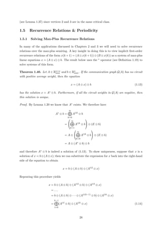
24](https://image.slidesharecdn.com/10d08b3f-967c-4123-bade-f0ef8267a94d-151012204735-lva1-app6891/85/Thesis_JR-29-320.jpg)
![eigenspace of A is given by
V (A) =
Nc(A)
r=1
αr ⊗ [A∗
λ]·jc
r
: αr ∈ Rmax, at least one αr finite
for any set of representative vertices {jc
1, . . . , jc
Nc(A)} of the critical classes of A.
Proof. By Lemma 1.36 we know that any eigenvector of A is a linear combination of the columns
[A∗
λ]·j, for j ∈ Vc(A). However, by Lemma 1.37 we know that the columns [A∗
λ]·j for j in some
critical class Vc
r (A) are all colinear. Therefore to build any eigenvector we only need one column
corresponding to each critical class, and so it suffices to take the sum over a set of representative
vertices of the critical classes of A.
Theorem 1.39. No column [A∗
λ]·i, for i ∈ Vc(A), can be expressed as a linear combination of
columns [A∗
λ]·jc
r
, where jc
r varies over the representative vertices of critical classes distinct from
that of i.
Proof. The proof of this statement requires substantial groundwork which we do not have the
space to include. For all the details and a full proof, readers are referred to theorem 3.101 in
[2].
Theorem 1.39 above tells us that we cannot simplify any further the expression for V (A) given
in Theorem 1.38. It also tells us that for an irreducible matrix A, the columns [A∗
λ]·jc
r
, where
{jc
1, . . . , jc
Nc(A)} is a set of representative vertices of the critical classes of A, form a basis for
the eigenspace V (A).
1.4.3 A Worked Example
Consider the matrix
A =
ε −2 ε 6
1 ε 4 ε
ε 8 ε ε
ε 5 ε 6
Thus G(A) looks like
25](https://image.slidesharecdn.com/10d08b3f-967c-4123-bade-f0ef8267a94d-151012204735-lva1-app6891/85/Thesis_JR-30-320.jpg)
![1
4
2 3
1 8
-2
5
4
6
6
Figure 1.1: Communication graph of the matrix A given above. Vertices are represented as
circles and numbered 1-4 by convention. Edges are present only if the corresponding entry in
A is finite, in which case this value specifies the edge weight.
We can see that G(A) is strongly connected, so A is irreducible. Thus by Theorem 1.30, A has
a unique eigenvalue λ given by the maximal average circuit weight in G(A). The elementary
circuits and their average weights are
c1 = (1, 2, 1) |c1|w/|c1|l = (1 ⊗ −2)/2 = −0.5
c2 = (1, 2, 4, 1) |c2|w/|c2|l = (1 ⊗ 5 ⊗ 6)/3 = 4
c3 = (2, 3, 2) |c3|w/|c3|l = (8 ⊗ 4)/2 = 6
c4 = (4, 4) |c4|w/|c4|l = (6)/1 = 6
and therefore λ = max{−0.5, 4, 6, 6} = 6. Circuits c3 and c4 are critical, so the critical graph
Gc(A) looks like
2 3 4
8
4
6
Figure 1.2: Critical graph of the matrix A given above. Both the circuits have maximal average
weight of 6. The other circuits present in Figure 1.1 are no longer included because they are
not critical (their average weight is not maximal).
We can see that Vc(A) = {2, 3, 4}, and Gc(A) has two critical classes with vertex sets Vc
1(A) =
{2, 3} and Vc
2(A) = {4} respectively. Thus {jc
1 = 2, jc
2 = 4} is a set of representative vertices of
the critical classes of A. Now, using that [Aλ]ij = aij − λ, we have
Aλ =
ε −8 ε e
−5 ε −2 ε
ε 2 ε ε
ε −1 ε e
and either by inspection of G(Aλ), or by using Lemma 1.17 and computing A⊗1
λ , A⊗2
λ , A⊗3
λ and
26](https://image.slidesharecdn.com/10d08b3f-967c-4123-bade-f0ef8267a94d-151012204735-lva1-app6891/85/Thesis_JR-31-320.jpg)
![A⊗4
λ , we can see that
A+
λ =
−6 −1 −3 e
−5 e −2 −5
−3 2 e −3
−6 −1 −3 e
Similarly, by using Lemma 1.20 (or by simply replacing any non-zero diagonal values in A+
λ
above by e), we obtain
A∗
λ =
e −1 −3 e
−5 e −2 −5
−3 2 e −3
−6 −1 −3 e
Now by theorems 1.38 and 1.39, the columns [A∗
λ]·2 & [A∗
λ]·4 form a basis for the eigenspace of
A, i.e.
V (A) =
α1 ⊗
−1
e
2
−1
α2 ⊗
e
−5
−3
e
: α1, α2 ∈ Rmax, at least one αr finite
For example, if we take α1 = −2, α2 = 1 we get
v := −2 ⊗
−1
e
2
−1
1 ⊗
e
−5
−3
e
=
−3
−2
e
−3
1
−4
−2
1
=
1
−2
e
1
and we can easily verify that this is indeed an eigenvector of A, associated with the unique
eigenvalue λ = 6:
A ⊗ v =
ε −2 ε 6
1 ε 4 ε
ε 8 ε ε
ε 5 ε 6
1
−2
e
1
=
7
4
6
7
= 6 ⊗
1
−2
e
1
= λ ⊗ v
Finally, we can observe that
[A∗
λ]·3 =
−3
−2
e
−3
= −2 ⊗
−1
e
2
−1
= −2 ⊗ [A∗
λ]·2
That is, columns [A∗
λ]·2 and [A∗
λ]·3 are scalar multiples of each other, which we would expect
27](https://image.slidesharecdn.com/10d08b3f-967c-4123-bade-f0ef8267a94d-151012204735-lva1-app6891/85/Thesis_JR-32-320.jpg)
![If c is a critical circuit of length l in G(A⊗k) then there is a corresponding critical circuit c of
length k ×l in G(A). This circuit must be in Gc(A) (because it is critical), which in turn implies
that c is a critical circuit in G((Ac)⊗k). Hence, it follows that Gc((Ac)⊗k) ⊇ Gc(A⊗k). The other
inclusion is proved in the same way.
Lemma 1.46. Let A ∈ Rn×n
max be an irreducible matrix with cyclicity σ = σ(A). Then the
cyclicity of the matrix A⊗σ is equal to one.
Proof. Firstly, suppose the critical matrix Ac is irreducible. By the remarks prior to Lemma 1.45
we know that the cyclicity of Ac and that of its communication graph is equal to σ, so by Lemma
1.43, after a suitable relabelling of vertices, (Ac)⊗σ corresponds to a block diagonal matrix with
square diagonal blocks that are irreducible and have graph cyclicity one. However, by Lemma
1.45 with k = σ, we have that Gc((Ac)⊗σ) = G((Ac)⊗σ), and therefore the communication graph
of each of the diagonal blocks of (Ac)⊗σ coincides with its critical graph. Thus for each diagonal
block both cyclicities coincide, and therefore both are one.
If Ac is reducible then the same process can be done for each of the critical classes of Gc(A) with
their individual cyclicities. According to Definition 1.41, the least common multiple of these
cyclicities equals σ, the matrix cyclicity of A. Noting that σ is a multiple of σG(A), it follows
from Corollary 1.44 that each diagonal block of (Ac)⊗σ corresponds to a block diagonal matrix
with square diagonal blocks that are irreducible and have cyclicity one. Note that if Gc(A) does
not cover all the vertices of G(A) then we must augment the overall block diagonal matrix with
a square block with entries equal to ε in order to keep it the same size as the original matrix A.
In both cases it follows that each diagonal block of the block diagonal matrix corresponding to
(Ac)⊗σ is irreducible and has cyclicity one. Taking the least common multiple of all cyclicities,
this means that the cyclicity of the whole matrix (Ac)⊗σ is equal to one, and therefore the graph
cyclicity of Gc((Ac)⊗σ) is also equal to one. But by Lemma 1.45 with k = σ, this graph is the
same as Gc(A⊗σ), which therefore must also have cyclicity one. Thus A⊗σ has matrix cyclicity
one, which completes the proof.
We now state a fundamental theorem, the proof of which can be found in [4].
Theorem 1.47. Let β1, . . . , βq ∈ N be such that gcd{β1, . . . , βq} = 1. Then there exists N ∈ N
such that for all k ≥ N there exist n1, . . . , nq ∈ N0 such that k = (n1 × β1) + · · · + (nq × βq).
We finally state and prove one last prerequisite result which is essentially a special case of the
theorem that follows. It turns out that the generalisation is relatively straightforward, so in
proving this lemma we will have done most of the work in proving the main result.
Lemma 1.48. Let A ∈ Rn×n
max be an irreducible matrix with unique eigenvalue e and cyclicity
one. Then there exists N ∈ N such that
A⊗(k+1)
= A⊗k
33](https://image.slidesharecdn.com/10d08b3f-967c-4123-bade-f0ef8267a94d-151012204735-lva1-app6891/85/Thesis_JR-38-320.jpg)
![for all k ≥ N.
Proof. The proof comes in three stages. We show that there exists N ∈ N such that for all
k ≥ N:
1. [A⊗k]ii = [A+]ii = e for all i ∈ Vc(A),
2. [A⊗k]ij = [A+]ij for all i ∈ Vc(A) and j ∈ {1, . . . , n},
3. [A⊗k]ij = l∈Vc(A)[A+]il ⊗ [A+]lj for all i, j ∈ {1, . . . , n}.
The result then follows immediately from statement 3 since the right hand side does not depend
on k.
Statement 1. Consider i ∈ Vc(A). Then there is a critical class of Gc(A), say Gc
1(A) =
(Vc
1(A), Ec
1(A)), such that i ∈ Vc
1(A). Since the cyclicity of matrix A is one, it follows that
the cyclicity of graph Gc
1(A) is equal to one too. Hence there exist circuits in Gc
1(A), say
c1, . . . , cq, whose lengths have a greatest common divisor equal to one. Since Gc
1(A) is a critical
class it must be strongly connected, and therefore there exists a circuit α in Gc
1(A) that passes
through i and through all circuits c1, . . . , cq (i.e. α ∩ cj = ∅ ∀j = 1, . . . , q).
Now, by Theorem 1.47, there exists N ∈ N such that for each k ≥ N, there exist n1, . . . , nq ∈ N0
such that
k = |α|l + (n1 × |c1|l) + · · · + (nq × |cq|l).
For these n1, . . . , nq, we can construct a circuit passing through i, built from circuit α, n1 copies
of circuit c1, n2 copies of circuit c2 and so on, up to nq copies of circuit cq. Clearly this circuit
is in Gc
1(A), so it must be critical with weight e. Since the maximal average circuit weight in
G(A) is e, it follows that [A⊗k]ii = e for all k ≥ N, which, by the definition of A+, also implies
that [A+]ii = e, as required.
Statement 2. By the definition of A+ there exists l ∈ N such that [A⊗l]ij = [A+]ij. In fact, since
the eigenvalue of A is e, it follows from Lemma 1.17 that l ≤ n. From statement 1, for k large
enough, i ∈ Vc(A) and j ∈ {1, . . . , n}, we then have
[A⊗(k+l)
]ij ≥ [A⊗k
]ii ⊗ [A⊗l
]ij = [A⊗l
]ij = [A+
]ij.
In addition, clearly we also have
[A+
]ij =
∞
m=1
[A⊗m
]ij ≥ [A⊗(k+l)
]ij ≥ [A+
]ij,
so by replacing k + l with k, it therefore follows that [A⊗k]ij = [A+]ij for all i ∈ Vc(A) and
j ∈ {1, . . . , n}, with k large enough. This is what we wanted to prove.
Statement 3. Following the same lines as in the proof of statement 2, we can also show that
[A⊗m]ij = [A+]ij for all i ∈ {1, . . . , n}, j ∈ Vc(A) and with m large enough. Together, take k
34](https://image.slidesharecdn.com/10d08b3f-967c-4123-bade-f0ef8267a94d-151012204735-lva1-app6891/85/Thesis_JR-39-320.jpg)
![and m large enough such that [A⊗k]il = [A+]il and [A⊗m]lj = [A+]lj for all l ∈ Vc(A). Then
[A⊗(k+m)
]ij ≥ [A⊗k
]il ⊗ [A⊗m
]lj = [A+
]il ⊗ [A+
]lj,
for all l ∈ Vc(A). By replacing k + m with k, it follows that for k large enough
[A⊗k
]ij ≥
l∈Vc(A)
[A+
]il ⊗ [A+
]lj.
Now let the maximal average weight of a non-critical circuit (i.e. a circuit not passing through
any vertex in Vc(A)) be δ. Then the weight of a path from j to i of length k + 1 in G(A) not
passing through any vertex in Vc(A) can be bounded above by [A+]ij + (k × δ) = [A+]ij ⊗ δ⊗k,
since such a path consists of an elementary path from j to i (whose weight is bounded above by
[A+]ij) and at most k non-critical circuits (whose weights are each bounded above by δ). Since
the maximal average circuit weight in G(A) is e we must have δ < e, and so for k large enough
[A+
]ij ⊗ δ⊗k
≤
l∈Vc(A)
[A+
]il ⊗ [A+
]lj.
Indeed, the right-hand side is fixed, while the left-hand side tends to ε as k → ∞. Hence for k
large enough we have that
[A⊗k
]ij =
l∈V(A)
[A+
]il ⊗ [A+
]lj =
l∈Vc(A)
[A+
]il ⊗ [A+
]lj,
for all i, j = 1, . . . , n.
We can now state and prove the main theorem of this section.
Theorem 1.49. Let A ∈ Rn×n
max be an irreducible matrix with unique eigenvalue λ and cyclicity
σ := σ(A). Then there exists N ∈ N such that
A⊗(k+σ)
= λ⊗σ
⊗ A⊗k
for all k ≥ N.
Proof. Consider the matrix B := (Aλ)⊗σ. Recall that σ is the cyclicity of the critical graph of
A, which is a multiple of the cyclicity of the communication graph G(A). By Corollary 1.44,
after a suitable relabelling of the vertices of G(A), matrix B is a block diagonal matrix with
square diagonal blocks whose communication graphs are strongly connected and have cyclicity
one. By Lemma 1.46 we have that the cyclicity of B is one, which implies that the cyclicity of
each of its diagonal blocks is one. Hence by applying Lemma 1.48 to each diagonal block, it
ultimately follows that there exists M ∈ N such that B⊗(l+1) = B⊗l for all l ≥ M. That is,
(Aλ)⊗σ
⊗(l+1)
= (Aλ)⊗σ
⊗l
,
35](https://image.slidesharecdn.com/10d08b3f-967c-4123-bade-f0ef8267a94d-151012204735-lva1-app6891/85/Thesis_JR-40-320.jpg)
![which can further be written as (Aλ)⊗(l×σ+σ) = (Aλ)⊗(l×σ), or
A⊗(l×σ+σ)
= λ⊗σ
⊗ A⊗(l×σ)
,
for all l ≥ M. Finally, note that A⊗(l×σ+j+σ) = λ⊗σ ⊗A⊗(l×σ+j) for any 0 ≤ j ≤ σ−1, implying
that for all k ≥ N := M × σ it follows that
A⊗(k+σ)
= λ⊗σ
⊗ A⊗k
,
as required.
Theorem 1.49 can be seen as the max-plus analogue of the Perron-Frobenius theorem in con-
ventional linear algebra. Strictly speaking it is the normalised matrix Aλ that exhibits periodic
behaviour, since the unique eigenvalue of Aλ is e = 0, and then A
⊗(k+σ)
λ = A⊗k
λ for k sufficiently
large. However, we use the term ‘periodic’ to describe the more general behaviour seen here.
Note that the cyclicity of A is the smallest possible length of such periodic behaviour (see [2] for
the proof of this). For our purposes, we now move on to applying this result to the recurrence
relations studied in Section 1.5.1.
Recall the form of the basic first-order recurrence relation
x(k + 1) = A ⊗ x(k), k ≥ 0, (1.20)
which has the solution
x(k) = A⊗k
⊗ x(0).
We can apply Theorem 1.49 in this context to give us that for k sufficiently large:
x(k + σ(A)) = A⊗(k+σ(A))
⊗ x(0)
= λ⊗σ(A)
⊗ A⊗k
⊗ x(0)
= λ⊗σ(A)
⊗ x(k).
That is, the solution x(k) is periodic with period σ(A). If we interpret k as a time index,
then also by Theorem 1.49, the solution enters this periodic regime after N =: t(A) time steps,
where we call t(A) is the transient time of A. In particular, if A has cyclicity equal to 1 then
x(k+1) = A⊗x(k) = λ⊗x(k) ∀k ≥ t(A), and so for k sufficiently large x(k) effectively becomes
an eigenvector of A. In other words, after t(A) time steps, x(k) behaves like an eigenvector, and
the effect of the initial condition x(0) has died out.
Note that the transient time of a matrix can be large even for systems of small dimension. For
example, the matrix A defined by
A =
−1 −N
e e
36](https://image.slidesharecdn.com/10d08b3f-967c-4123-bade-f0ef8267a94d-151012204735-lva1-app6891/85/Thesis_JR-41-320.jpg)
![where N ∈ {2, 3, . . . } has transient time t(A) = N, while its cyclicity is clearly 1.
Finally, we make some observations regarding the growth rate of the solution x(k). Note that
if we take x(0) = v in (1.20), where v is an eigenvector of A, then we immediately obtain that
for all j = 1, . . . , n:
lim
k→∞
xj(k)
k
= λ,
where λ is the unique eigenvalue of A. By applying Theorem 1.49 it should be clear that this
holds true for any initial value x(0) and not just for eigenvectors; indeed this result is proved
in [13]. We therefore say that the solution has an asymptotic growth rate of λ. Assuming
irreducibility, all recurrence relations over max-plus exhibit this behaviour, regardless of the
choice of the matrix A!
37](https://image.slidesharecdn.com/10d08b3f-967c-4123-bade-f0ef8267a94d-151012204735-lva1-app6891/85/Thesis_JR-42-320.jpg)
![Chapter 2
Petri Nets and Timed Event Graphs
2.1 A Motivating Example
The following example is adapted from chapter 1 of [2]. Consider a manufacturing system
consisting of three machines M1, M2 and M3, which produces three kinds of parts P1, P2 and
P3 according to different product mixes. The manufacturing process for each part is depicted
below.
M1 M2 M3
P2
P3
P1
Figure 2.1: Manufacturing Process for each part. Grey boxes represent the three machines;
arrows represent the routes that the different parts must take in their respective manufacture.
Processing times are different for each machine and each part, and are given in the following
table:
P1 P2 P3
M1 - 1 5
M2 3 2 3
M3 4 3 -
Table 2.1: Processing times for each part at each machine (arbitrary time units). Blank entries
correspond to combinations of machine & part that do not form part of the manufacturing
process.
Parts are carried through the manufacturing process on a limited number of pallets. We make
38](https://image.slidesharecdn.com/10d08b3f-967c-4123-bade-f0ef8267a94d-151012204735-lva1-app6891/85/Thesis_JR-43-320.jpg)
![the following assumptions:
1. Only one pallet is available for each part type.
2. Once production of a part is completed, it is removed from its respective pallet and the
pallet returns to the beginning of the production line.
3. There are no set-up times or traveling times between machines.
4. The sequencing of part types on the machines is fixed, and for M1 is (P2, P3), for M2
(P1, P2, P3) and for M3 (P1, P2).
Assumption (3) gives no loss of generality since if set-up times or traveling times did exist,
we could combine them with the processing time at the appropriate machine. Assumption (4)
means that machines have to wait for the appropriate part rather than starting work on any
part that arrives first (see below for an example). This may or may not be realistic; extensions
to the theory presented below in which this assumption is dropped are discussed in chapter 9
of [2].
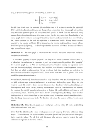
We can model the time evolution of this system by considering the time that each machine starts
working on the k-th part of type i, for i = 1, 2, 3 and k ∈ N. There are seven combinations of
machines and parts, so we define x(k) = (x1(k), . . . , x7(k)) as follows:
Variable xi(k) Definition
x1(k) time that M1 starts working on the k-th unit of P2
x2(k) time that M1 starts working on the k-th unit of P3
x3(k) time that M2 starts working on the k-th unit of P1
x4(k) time that M2 starts working on the k-th unit of P2
x5(k) time that M2 starts working on the k-th unit of P3
x6(k) time that M3 starts working on the k-th unit of P1
x7(k) time that M3 starts working on the k-th unit of P2
Table 2.2: Definitions of each entry of the state vector x(k), for k ∈ N.
By examining the production process, work by each machine on the (k+1)-st part is constrained
in the following way:
x1(k + 1) ≥ max x7(k) + 3, x2(k) + 5
x2(k + 1) ≥ max x5(k) + 3, x1(k + 1) + 1
x3(k + 1) ≥ max x6(k) + 4, x5(k) + 3
x4(k + 1) ≥ max x3(k + 1) + 3, x1(k + 1) + 1
x5(k + 1) ≥ max x2(k + 1) + 5, x4(k + 1) + 2
x6(k + 1) ≥ max x3(k + 1) + 3, x7(k) + 3
x7(k + 1) ≥ max x6(k + 1) + 4, x4(k + 1) + 2
39](https://image.slidesharecdn.com/10d08b3f-967c-4123-bade-f0ef8267a94d-151012204735-lva1-app6891/85/Thesis_JR-44-320.jpg)
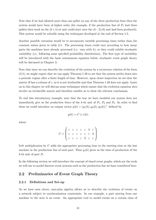
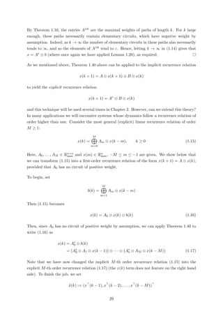
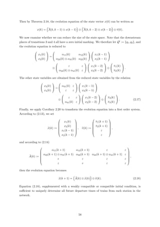
![and let A(k), k ∈ Z, be the (|Q | × M) × (|Q | × M) matrix defined by the relation
A(k) :=
A(k + 1, k) A(k + 1, k − 1) . . . . . . A(k + 1, k + 1 − M)
E E . . . E E
E E
...
... E
...
... E E E
E . . . E E E
(2.14)
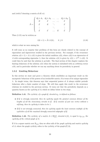
where E denotes the |Q | × |Q | matrix of ε. Finally, let v(k) be the (|Q | × M)-dimensional
vector
v(k) :=
v(k + 1)
ε
...
ε
.
Then we can state the following corollary, which gives the standard form of the basic autonomous
equation:
Corollary 2.20. The extended state space vector x(k) satisfies the (M × |Q |)-dimensional
first-order evolution equation
x(k + 1) = A(k) ⊗ x(k) ⊕ v(k), (2.15)
for k ∈ Z.
Proof. This technique is standard and the result follows immediately from conducting the ap-
propriate matrix multiplications.
Once again, in the particular case of a compatible initial condition, these equations read
x(k + 1) = A(k) ⊗ x(k)
provided one uses the appropriate continuation of xj(k) for k ≤ 0.
Note that we can associate the standard form basic autonomous equation given in Corollary
2.20 with an event graph which is once again equivalent to the original event graph, but this
time with initial marking equal to 1 everywhere. An algorithm for obtaining the derived graph
can be found in [2].
2.3.4 Behaviour of the Solution
Assume for a moment that the holding times of our event graph are constant and that we forgo
the state space reduction described above. We have that the evolution of a live autonomous
FIFO timed event graph (G, µ), supplemented with a compatible initial condition, is described
54](https://image.slidesharecdn.com/10d08b3f-967c-4123-bade-f0ef8267a94d-151012204735-lva1-app6891/85/Thesis_JR-59-320.jpg)
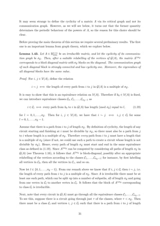
![by the recurrence relation
x(k) =
M
m=0
A(m) ⊗ x(k − m)
and we have just shown that the same equation in standard form
x(k + 1) = A ⊗ x(k)
equivalently describes the evolution of the system, and can be associated with an event graph G
which is equivalent to G. Since we assume that G is strongly connected it can also be assumed
that G is strongly connected, provided unnecessary transitions (not involved in circuits) be
cancelled. Hence we can assume that A is irreducible. We can therefore apply Theorem 1.49 to
see that after a finite period of time, the solution will enter a periodic regime with period t(A)
and asymptotic growth rate λ, where λ is the unique eigenvalue of A. An interpretation of this
is that on average, each transition fires once every λ units of time, i.e. the long-run throughput
of each transition is 1/λ, thus achieving some sort of stationarity.
A nice result given in [2] is that the value λ can be obtained directly from the original event
graph G, provided we modify slightly our definition of path lengths and weights. To be specific,
in the case of an event graph we can think of places as edges with weight equal to their holding
time, and length equal to the number of tokens in their initial marking. Using this definition,
λ is then equal to the maximal average circuit weight in G.
The behaviour of the solution x(k) in the case of variable holding times is more difficult to
describe. It can be shown that if there are sufficiently long sub-intervals for which the holding
times are constant then the solution exhibits periodicity within each of these intervals. This
can be seen in our simple example to which we return below.
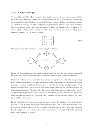
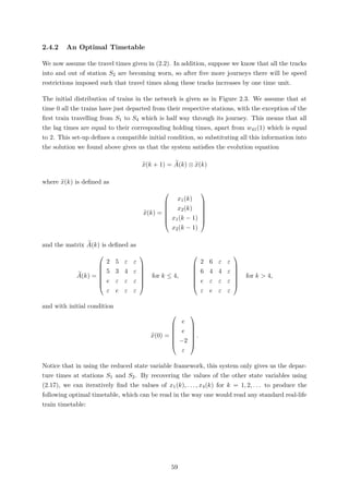
2.4 A Simple Example Revisited
2.4.1 General Solution
Consider the example given in Section 2.2.2, and suppose that we extend to the model to allow
for variable travel times between stations. We denote the travel time of the k-th train between
Sj and Sl by αlj(k). Similarly, wlj(k) denotes the remaining travel time of the k-th train
between Sj and Sl present at time 0 (and is equal to ε if no such train exists). We assume that
the initial marking is the same as that given in Figure 2.3. The aim of this section is to apply
the theory developed above to find a timetable describing the optimal departure times of trains
at each station.
Under the assumption that the holding times are such that the event graph is FIFO, according
55](https://image.slidesharecdn.com/10d08b3f-967c-4123-bade-f0ef8267a94d-151012204735-lva1-app6891/85/Thesis_JR-60-320.jpg)
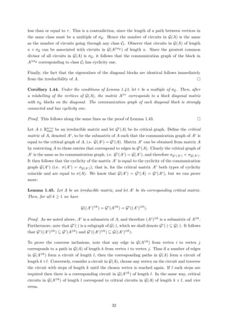
![Departure Times
S1 - 0 5 12 17 24 29 37 43 51 57
S2 - 0 7 12 19 24 31 37 45 51 59
S3 - 2 7 14 19 26 31 39 45 53 59
S4 2 4 9 16 21 28 33 41 47 55 61
Table 2.3: Optimal Timetable of the Train Network. Recall that synchronisation results in
departures from stations coinciding, so the times given here refer to departures from each
station in all directions (for example, at time 5 one train departs on the inner-city loop at S1,
a second departs for S3 and a third departs for S3).
Note that we have shifted the variable k by 1 and 2 for the third and fourth rows respectively
so that the departure times line up nicely. Specifically, the columns in Table 2.3 represent the
vectors (x1(k), x2(k), x3(k + 1), x4(k + 2)) for k = −1, 0, 1, . . . , 9. This results in a sequence
of departure times that is increasing (when read down and then across). This is purely for
presentational reasons - we opt to make the departure timetable easy to read for someone
travelling through the network starting at station S1.
Notice that as per Section 2.3.4, the solution settles into a temporary periodic regime for k ≤ 5,
with asymptotic growth rate λ1 = 6 and transient time 2. λ1 here corresponds to the maximal
average weight of all the circuits of the event graph given in Figure 2.3 (where we think of the
holding times as weights and the number of tokens in the initial marking as lengths; see Section
2.3.4). For k > 5, the solution enters a second periodic regime with asymptotic growth rate
λ2 = 7. λ2 once again corresponds to the maximal average weight of all the circuits of the
original event graph but with the holding times updated to reflect the adjusted travel times.
There is an additional transient period of 2 time units (k = 6 to 8) during which the solution is
temporarily aperiodic.
In both cases the period is equal to 2, which therefore must be the cyclicity of the matrix A (k)
for which the whole system is described by the evolution equation x(k + 1) = A (k) ⊗ x(k) (i.e.
if we had not reduced the state space). We know that this matrix must be irreducible (again
see the discussion in Section 2.3.4), but it is not immediate that the support of its critical graph
(i.e. the set of edges (i, j) ∈ Ec(A (k)) for which [A (k)]ji = ε) is invariant under changes in k.
In fact, in this case we can show that it is, which explains why the cyclicity does not change for
the second periodic regime.
2.5 The Non-autonomous Case
This section focuses on FIFO timed event graphs that are non-autonomous; that is, event graphs
that include source transitions. Whilst we require one or two additional concepts, a lot of the
theory is analogous to the autonomous case and we therefore omit proofs whenever appropriate.
Firstly, we define a new class of transitions known as input transitions.
Definition 2.21. An input transition consists of a source transition and a non-decreasing
60](https://image.slidesharecdn.com/10d08b3f-967c-4123-bade-f0ef8267a94d-151012204735-lva1-app6891/85/Thesis_JR-65-320.jpg)
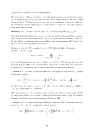
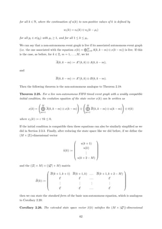
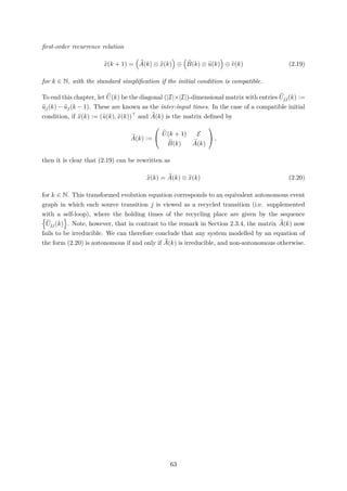
![Chapter 3
Stochastic Event Systems Over
Max-plus
3.1 Introduction & Stochastic Background
In this chapter we consider stochastic FIFO event graphs; that is, FIFO event graphs in which
the holding times and lag times are random variables rather than predetermined constants. We
are interested in the conditions under which these graphs enter a stationary regime. Most of the
material in this chapter is taken from [1], [2] and [12]. We begin by laying some foundations of
Ergodic theory and describing the statistical assumptions we will use throughout. The manner
in which we introduce the concepts below may be surprising - specifically, what we state as
definitions are actually theorems which follows from the classical definition of ergodicity. Whilst
the reader may be more familiar with the latter approach, we find that in the context of max-plus
stochastic event systems it is intuitively helpful to proceed in this way.
Definition 3.1. Let (Ω, F, P) be a probability space. The mapping θ : Ω → Ω is a shift operator
on (Ω, F, P) if it is bijective and measurable, and if it is such that P is left invariant by θ, namely
E[f] = E[f ◦ θ] for all measurable and integrable functions f : Ω → R (where E represents the
expectation w.r.t. P).
Definitions 3.2. Let θ be a shift operator on (Ω, F, P).
(i) A sequence of R-valued random variables a(k, ω) k∈Z defined on (Ω, F, P) is θ-stationary
if a(k, ω)
d
= a(0; θk(ω)) ∀k ≥ 0, where θk is the composition of θ by itself k times.
(ii) θ is ergodic if the almost sure (a.s.) limit
lim
k→∞
1
k
k
l=1
f ◦ θ l
(ω) = E[f]
holds for all measurable and integrable functions f : Ω → R.
64](https://image.slidesharecdn.com/10d08b3f-967c-4123-bade-f0ef8267a94d-151012204735-lva1-app6891/85/Thesis_JR-69-320.jpg)
![A simple example of an ergodic sequence of random variables is a sequence of independent
identically distributed (i.i.d.) random variables, and this will often be the obvious choice for
the sequence of holding times in the modelling of real-life systems such as rail networks.
Notation. Recall from Definition 1.3 that for a, b ∈ Rmax, we say a ≤ b if a ⊕ b = b. In this
chapter we introduce the notation a ∧ b to mean the greatest lower bound of a and b, i.e.
a ≤ b ⇐⇒ a ⊕ b = b ⇐⇒ a ∧ b = a. (3.1)
The ∧ operation is associative, commutative and idempotent but it does not have an identity
element, and does not always distribute over ⊗. For our purposes, we can think of a∧b to mean
min {a, b}.
We must take extra care to ensure that some fundamental concepts of probability are applicable
in the max-plus setting. For example, if X is a random variable taking values in Rmax defined
on a probability space (Ω, F, P) then it may take the value ε with positive probability, which
confuses the idea of integrability. We therefore call X ∈ Rmax integrable if X ⊕ e and
X ∧ e are both integrable, and if E[X ⊕ e] is finite. The expected value of X is then given by
E[X] = E[X ⊕e] ⊗ E[X ∧e]. Moreover, a random matrix A ∈ Rn×m
max (i.e. a matrix whose entries
are random variables taking values in Rmax) is called integrable if the entries aij are integrable
∀i, j, and its expected value is given by the matrix E[A] with entries E[A] ij = E[aij].
3.2 Statistical Assumptions
In this chapter we consider the max-plus evolution equation
x(k + 1) = A(k) ⊗ x(k), k ∈ Z (3.2)
with initial condition x(0) = x0. We will often stress the dependence of x(k) on the initial
condition by writing x(k; x0). We assume that A(k) k∈Z is a sequence of random matrices
defined on a common probability space (Ω, F, P) endowed with an ergodic shift operator θ, and
that x0 is also a random variable defined on this space. If we let
A := A(0) (3.3)
then θ-stationarity gives us that A(k)
d
= A ◦ θ k ∀k ∈ Z. We assume in addition that each entry
of A is either a.s. equal to ε or non-negative and integrable, and that each diagonal of A is
non-negative.
Throughout the rest of this chapter, what we have described above will be known as the SENI
framework (stationary, ergodic, non-negative and integrable). Note that the assumptions of the
SENI framework mean that the sequence of matrices A(k) has fixed support (i.e. the topologies
of the communication graphs G(A(k)) are non-random and do not vary with k). A formal
definition is given below.
65](https://image.slidesharecdn.com/10d08b3f-967c-4123-bade-f0ef8267a94d-151012204735-lva1-app6891/85/Thesis_JR-70-320.jpg)
![Definition 3.3. The sequence of matrices A(k) ∈ Rn×n
max has fixed support if the probability that
[A(k)]ij equals ε is either 0 or 1 and does not depend on k.
The remainder of this section is devoted to showing that both autonomous and non-autonomous
FIFO stochastic event graphs are described by an evolution equation which falls into the SENI
framework.
The Autonomous Case By the remark that follows Corollary 2.20, for an autonomous FIFO
timed event graph with a compatible initial condition, the extended state space vector x(k)
satisfies the evolution equation
x(k) = A(k) ⊗ x(k)
which is of the form (3.2). Suppose in addition that the holding times αi(k) and the lag times
wi(k), i = 1, . . . , |P|, are random variables defined on a common probability space endowed
with an ergodic shift operator θ, and that the sequence αi(k) k∈Z is θ-stationary. Then it is
easily verified that the matrices A(k) satisfy the θ-stationarity property and that each entry of
A := A(0) is either a.s. equal to ε or non-negative and integrable. Furthermore, by the FIFO
assumption we have that xj(k + 1) ≥ xj(k) ∀k, and therefore Ajj(k) ≥ e for all j. Therefore,
under the appropriate statistical assumptions, any autonomous FIFO stochastic event graph
with compatible initial condition falls into the SENI framework.
The Non-autonomous Case By the remark that follows Corollary 2.26, the evolution of a non-
autonomous FIFO timed event graph with a compatible initial condition is described by the
equation
x(k) = A(k) ⊗ x(k)
which is also of the form (3.2). If the holding times αi(k) and the inter-input times Ujj(k)
are sequences of non-negative and integrable random variables satisfying θ-stationarity, then it
is again straightforward to check that the matrices A(k) are also θ-stationary. The additional
conditions mentioned above also follow in the same way as the autonomous case. Therefore the
SENI framework also covers the non-autonomous case, provided we make additional assumptions
on the inter-input times.
3.3 Asymptotic Firing Rates
In Section 2.3.4 we showed that in the case of constant holding times, any strongly connected
timed event graph will eventually reach a periodic regime in which each transition fires every
λ units of time (where λ is a constant determined by the event graph in question). The aim
of this section is to develop a corresponding theory for stochastic event graphs, i.e. to examine
whether the firing rates settle into a steady state distribution after a long period of time. We
will consider the case when the matrix A defined in (3.3) (herein assumed to be of dimension
n × n) is both a.s. irreducible and a.s. reducible, which is a well-defined distinction owing to
66](https://image.slidesharecdn.com/10d08b3f-967c-4123-bade-f0ef8267a94d-151012204735-lva1-app6891/85/Thesis_JR-71-320.jpg)
![the assumption of fixed support within the SENI framework. This corresponds to stochastic
event graphs which are a.s. strongly connected and a.s. not strongly connected respectively.
We begin with some new notation.
Notation. For A ∈ Rn×m
max , let
|A|⊕
:=
n
i=1
m
j=1
aij
and
|A|∧
:=
n
i=1
m
j=1
aij.
Thus |A|⊕ gives the maximal entry of A and |A|∧ gives the minimal entry of A.
Lemma 3.4. For all pairs of matrices A, B ∈ Rn×m
max such that the product A ⊗ B is well
defined, we have
|A ⊗ B|⊕ ≤ |A|⊕ ⊗ |B|⊕
|A ⊗ B|⊕ ≥ |A|∧ ⊗ |B|⊕
|A ⊗ B|⊕ ≥ |A|⊕ ⊗ |B|∧
and
|A ⊗ B|∧ ≥ |A|∧ ⊗ |B|∧
|A ⊗ B|∧ ≤ |A|∧ ⊗ |B|⊕
|A ⊗ B|∧ ≤ |A|⊕ ⊗ |B|∧
Proof. Since Aik ≤ |A|⊕ for all i, k,
i,j k
Aik ⊗ Bkj ≤ |A|⊕ ⊗
j,k
Bkj
= |A|⊕ ⊗ |B|⊕
The proofs of the other formulae follow similarly.
We now recall an important theorem from Ergodic theory known as Kingman’s Theorem on
subadditive ergodic processes. This will be used in the material below. We do not offer a proof
here; readers are referred to [14] for the full working.
Theorem 3.5 (Kingman’s subadditive ergodic theorem). Let ξm,n, m > n ∈ Z, be an integrable
random process defined on the probability space (Ω, F, P) such that
ξm,m+k
d
= ξ0,k ◦ θm
∀m ∈ Z, k > 0 (stationarity)
67](https://image.slidesharecdn.com/10d08b3f-967c-4123-bade-f0ef8267a94d-151012204735-lva1-app6891/85/Thesis_JR-72-320.jpg)
![and
ξm,n ≤ ξm,k + ξk,n a.s. ∀ m < k < n (subadditivity).
Assume in addition that there exists a positive constant c such that E[ξ0,k] ≥ −ck for all k > 0.
Then there exists a constant γ such that the following two equations hold:
lim
k→∞
ξ0,k
k
= γ a.s., lim
k→∞
E[ξ0,k]
k
= γ = inf
k
E[ξ0,k]
k
.
We now able to begin our task of characterising the asymptotic behaviour of the firing rates in
a stochastic event graph.
Theorem 3.6. Within the SENI framework, there exists a non-negative constant a ∈ Rmax
(known as the maximal Lyapunov exponent) such that, for all finite initial conditions x0, the
limit
lim
k→∞
|x(k; x0)|⊗1/k
⊕
= a (3.4)
holds almost surely. If the initial condition is integrable, in addition we have
lim
k→∞
E |x(k; x0)|⊗1/k
⊕
= lim
k→∞
E |x(k; x0)|⊕
⊗1/k
= a. (3.5)
Proof. Using the integrability assumptions of the SENI framework, we obtain by induction that
|x(k; e)|⊕ is integrable for all k ≥ 0. We therefore have
e ≤ E |x(k; e)|⊕ < ∞ ∀k ≥ 0.
Now let
ξm,m+k = |x(k; e)|⊕ ◦ θm
, m ∈ Z, k ≥ 0.
Since
|x(k, e)|⊕ = |A ◦ θk−1
⊗ · · · ⊗ A ⊗ e|⊕ = |A ◦ θk−1
⊗ · · · ⊗ A|⊕ ,
we obtain from Lemma 3.4 that for any k ≥ 1 and for all 0 ≤ p ≤ k:
|A ◦ θk−1
⊗ · · · ⊗ A ◦ θp
⊗ A ◦ θp−1
⊗ · · · ⊗ A|⊕ ◦ θm
≤ |A ◦ θk−1
⊗ · · · ⊗ A ◦ θp
|⊕ ◦ θm
⊗ |A ◦ θp−1
⊗ · · · ⊗ A|⊕ ◦ θm
;
that is, ξm,m+k ≤ ξm,m+p +ξm+p,m+k. Thus ξm,m+k is a non-negative and integrable subadditive
process. Using Theorem 3.5, we obtain
lim
k→∞
(ξ0,k)⊗1/k
= lim
k→∞
E (ξ0,k)⊗1/k
= a a.s.,
for some constant a < ∞, which concludes the proof for |x(k; e)|⊕ . Now, using that x(k) =
68](https://image.slidesharecdn.com/10d08b3f-967c-4123-bade-f0ef8267a94d-151012204735-lva1-app6891/85/Thesis_JR-73-320.jpg)
![A(k − 1) ⊗ · · · ⊗ A(0) ⊗ x0, by Lemma 3.4 we have that for all finite initial conditions x0 and
∀k ≥ 0:
|x(k; e)|⊕ ⊗ |x0|∧ ≤ |x(k; x0)|⊕ ≤ |x(k; e)|⊕ ⊗ |x0|⊕ .
Therefore
|x(k; e)|⊗1/k
⊕
⊗ |x0|⊗1/k
∧
≤ |x(k; x0)|⊗1/k
⊕
≤ |x(k; e)|⊗1/k
⊕
⊗ |x0|⊗1/k
⊕
(3.6)
for all k ≥ 0. We then immediately obtain property (3.4) by letting k tend to ∞. Similarly, if x0
is integrable then we can take expectations in (3.6) and use the fact that limk→∞ E[(ξ0,k)⊗1/k]
= a to obtain (3.5).
Note that we have only shown the existence of the constant a here, whereas in the deterministic
case we were able to specify its value. Computing exactly the maximal Lyapunov exponent of
products of matrices over the max-plus semiring is a long-standing problem, and only for a few
special cases are explicit formulae known [12]. However, it can be shown (see [2]) that if the
communication graph G(A) contains at least one circuit with two vertices i0, j0 in this circuit
such that E[Aj0i0 (k)] > e, then the maximal Lyapunov exponent a is strictly positive. This
corresponds to having a circuit with at least one place with positive mean holding time in the
stochastic event graph.
Theorem 3.6 tells us that |x(k)|⊕ grows like a⊗k. Using the same techniques we could prove an
analogous result for the growth rate of |x(k)|∧ which is also a constant b, called the minimal
Lyapunov exponent, and with b ≤ a. In the following section we examine the growth rate of the
individual state variables xj(k) within the SENI framework. In the irreducible case we show
that all state variables have the same asymptotic growth rate equal to the maximal Lyapunov
exponent defined above, and a similar result holds in the reducible case. This matches our
intuition that the speed with which a system operates is determined by its slowest component.
3.3.1 The Strongly Connected Case
We assume that A is a.s. irreducible. Recall that within the SENI framework we also assume
that the diagonal entries of A are a.s. non-negative. It is then easy to see that the matrices
G(k) := A(k + n − 1) ⊗ A(k + n − 2) ⊗ · · · ⊗ A(k), k ∈ Z
are such that Gij(k) ≥ e for all i, j = 1, . . . , n. This allows us to state the following corollary.
Corollary 3.7. Within the SENI framework, if the matrix A is irreducible, then for all finite
initial conditions x0 and for all j = 1, . . . , n, we have that
lim
k→∞
xj(k; x0)
⊗1/k
= a a.s.,
69](https://image.slidesharecdn.com/10d08b3f-967c-4123-bade-f0ef8267a94d-151012204735-lva1-app6891/85/Thesis_JR-74-320.jpg)
![where a is the maximal Lyapunov exponent of Theorem 3.6. If x0 is integrable, we also have
lim
k→∞
E xj(k; x0)
⊗1/k
= a.
Proof. From the remark above we obtain that xj(k; x0) ≥ xi(k − n; x0) for all i, j = 1, . . . , n
and k > n. This gives that
|x(k − n; x0)|⊕ ≤ xj(k; x0) ≤ |x(k; x0)|⊕ ∀j = 1, . . . , n
and the result follows by letting k tend to ∞ and applying Theorem 3.6. In the integrable case,
the proof of the convergence of the expectations in then immediate.
Corollary 3.7 tells us that in the case of a strongly connected stochastic event graph, all tran-
sitions have the same asymptotic firing rate. In this case the maximal Lyapunov exponent a is
also called the cycle time of the stochastic event graph, and its inverse a−1 is often referred to
as the throughput. By viewing the deterministic case of Chapter 2 as a special case, if A(k) = A
for all k ∈ N then the maximal Lyapunov exponent is simply the unique eigenvalue λ of A.
3.3.2 The General Case
If G(A) is not strongly connected then it can be decomposed into a number N(A) > 1 of
maximal strongly connected subgraphs (m.s.c.s.’s), in the same way as we did in Section 1.4 for
the critical graph Gc(A). Note that due to the assumptions of the SENI framework, the number
N(A) of m.s.c.s.’s and their topologies are non-random. Let Gr(A) = (Vr(A), Er(A)) denote the
r-th m.s.c.s. of G(A) and let jr := min j ∈ Vr(A) be the smallest numbered vertex in the r-th
m.s.c.s. We call {j1, . . . , jN(A)} a set of representative vertices of the m.s.c.s’s of G(A). We now
introduce some new notation and a simple definition.
Notation. For i ∈ V(A), let [i] denote the subset of vertices of the m.s.c.s. containing vertex i.
We then let x(i)(k) denote the subvector of x(k) associated with the vertex set [i]; that is, the
vector x(k) restricted to the entries corresponding to vertices in the m.s.c.s. containing vertex
i. Similarly, A(i)(j)(k) denotes the block extracted from A(k) by keeping rows associated with
the vertex set [i] and the columns associated with the vertex set [j].
Consistent with the notation used in Section 2.2, we let π+(i) be the set of ascendants of vertex
i; that is, the set of all vertices j such that a path exists from j to i (which by convention does
not include i itself). In addition, we let π∗(i) := {i} ∪ π+(i). We then let x(<i)(k) denote the
subvector of x(k) associated with the vertex set j∈π+(i)[j] (so x(<i)(k) denotes the restriction
of x(k) to the entries corresponding to vertices in the m.s.c.s’s of all the ascendants of vertex i,
not including the m.s.c.s. of i itself), and x(≤i)(k) denote the subvector of x(k) associated with
the vertex set j∈π∗(i)[j]. Finally, the matrices A(≤i)(≤j), A(<i)(<j) etc. are defined in the same
way.
Definition 3.8. The reduced graph of G(A) is the graph G(A) = (V(A), E(A)), with vertex set
V(A) := {j1, . . . , jN(A)} (one vertex per m.s.c.s.) and where (j1, j2) ∈ E(A) iff (k, l) ∈ E(A)
70](https://image.slidesharecdn.com/10d08b3f-967c-4123-bade-f0ef8267a94d-151012204735-lva1-app6891/85/Thesis_JR-75-320.jpg)
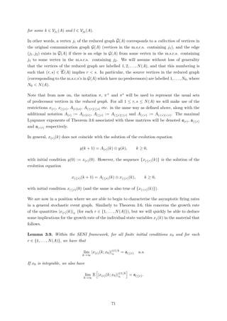
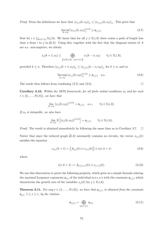
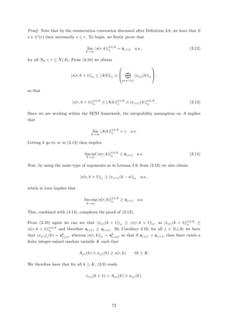
![Definition 3.12. A queuing system satisfies condition (A) if it only has one class of items, no
state-dependent service times, all queues are FCFS with blocking after service, and blocking is
resolved according to FBFU.
Note that a queuing system satisfying condition (A) is not necessarily max-plus linear (and so
cannot necessarily be represented by a stochastic event graph). However, as was our aim, it
turns out that (A) does specify the class of queuing system for which we can derive necessary
and sufficient conditions for max-plus linearity. In other words, reducing our analysis to queuing
systems of this type imposes no restriction in the context of stochastic event graphs.
The main reason for requiring the assumption (A) is that in a max-plus linear model we have no
information about the physical state of the system (in terms of queue lengths), and this means
that any dependence of the service times on the physical state cannot be incorporated. The
intuition should be reasonably clear and we choose to omit the details here; a full discussion
can be found in [12].
It is possible to derive a general recursive formula (in max-plus) describing the departure times
from queues in a queuing system satisfying (A). Once again, the full working can be found
in [12]. Having done this, it remains to identify conditions under which this formula can be
reduced to the form of the basic non-autonomous equation of Theorem 2.23 (or its autonomous
counterpart), which, as we have remarked above, will mean that the queuing system is max-plus
linear, and can be represented by a stochastic event graph. It boils down to whether the general
recursive formula is of finite order. A simple set of sufficient conditions for max-plus linearity
are summarised in the following result:
Theorem 3.13. A queuing system satisfying (A) is max-plus linear if it admits no internal
overtaking, and if all resequencing queues have a finite buffer.
The proof is not difficult but of considerable length, and can be found in [12].
3.4.2 Example: The G/G/1 Queue
The event graph in Figure 3.1 below represents the FIFO G/G/1 queue with an infinite buffer.
The G/G part states that both the interarrival times and holding times form general stationary
sequences. The 1 indicates that there is a single server (we assume that there is an infinite
buffer in front of the server). The input u1 into transition q1 features the external input stream
of items, p1 is the infinite buffer which stores the items to be served, q2 represents the single
server and the holding times in p2 represent the service times.
76](https://image.slidesharecdn.com/10d08b3f-967c-4123-bade-f0ef8267a94d-151012204735-lva1-app6891/85/Thesis_JR-81-320.jpg)
![q1 p1 q2
p2
Figure 3.1: Stochastic event graph representation of the G/G/1 queue with an infinite buffer.
Items enter the system via q1 and are stored in p1. Departures occur whenever q2 fires since this
will remove one token from the system. Note that p2 will never contain more than one token;
i.e. there can never be more than one person in service at any one time.
Notice that transition q2 has two upstream places but only one downstream place, so whenever
q2 fires (i.e. whenever the service of an item is completed) the total number of tokens in the
system reduces by one. Thus departures from the queue are modelled without the use of a sink
transition. By construction there will always be one token in place p2 (corresponding to the
item in service), whereas p1 could hold any number of tokens. The holding times in p1 are taken
to be e, so in particular they are non-random.
Recalling the notation of Chapter 2, notice that M = 1 and that both |Q | and |I| are equal
to 1. Hence the matrices A(k, k − 1) and B(k, k − 1) in the basic non-autonomous equation of
Theorem 2.23 are one-dimensional:
A(k, k − 1) = α(k) , B(k, k − 1) = (e).
Let A(k) = α(k+1). If the initial condition is weakly compatible (which will happen if u(1) ≥ e,
and the lag times w1, w2 satisfy w1 ≤ e, w2 ≤ α(1) and w1 ⊕ w2 ≥ e), then it is also compatible
(since each transition is followed by at most one place with non-zero initial marking), so the
basic non-autonomous equation gives us that the firing times satisfy
x(k + 1) = A(k) ⊗ x(k) ⊕ u(k), k ≥ 0,
provided we now take x(0) = w2 ⊗ α(1)⊗−1 and u(0) = w1.
3.4.3 Stability Analysis of Waiting Times
In this final section we present a celebrated result in the area of stochastic max-plus theory.
Recall that if in a G/G/1 queue the expected interarrival time is larger than the expected service
time, then the sequence of waiting times converges, independent of the initial condition, to a
unique stationary regime (see [16]). Our aim is to generalise this result to the waiting times in
open max-plus linear queuing systems.
Consider an open queuing system (i.e. one in which items can arrive from the outside world)
with one input transition and J queues, satisfying the conditions of Theorem 3.13. It is therefore
max-plus linear, and so the vector of departure times from each queue, denoted x(k), satisfies
77](https://image.slidesharecdn.com/10d08b3f-967c-4123-bade-f0ef8267a94d-151012204735-lva1-app6891/85/Thesis_JR-82-320.jpg)
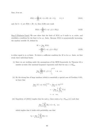
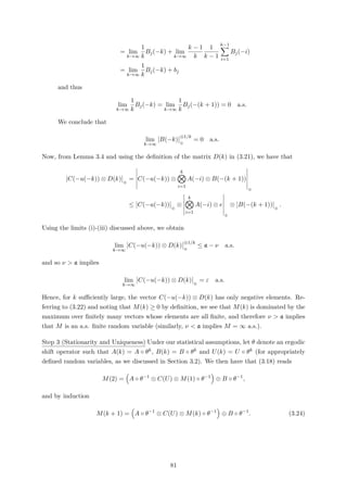
![Letting k tend to ∞ in (3.24) shows that
M = A ◦ θ−1
⊗ C(U) ⊗ M ⊕ B ◦ θ−1
;
that is, M is the stationary solution of (3.17), and it remains to show uniqueness. To do this,
let M(k, w) denote the vector of sojourn times at time 0 provided that the sequence is started
at −k and with initial vector w ∈ RJ
max. This gives
M(k, w) =
k
i=1
A(−i) ⊗ C(U(−i + 1)) ⊗ w ⊕
k−1
j=0
C(−u(−j)) ⊗ D(j).
Assuming that w has at least one finite element, we have that |w|⊕ < ∞. Following the same
argument as in step 2 above, we obtain that for ν > a:
lim
k→∞
k
i=1
A(−i) ⊗ C(U(−i + 1)) ⊗ w
⊕
= ε a.s.,
and so
lim
k→∞
k
i=1
A(−i) ⊗ C(U(−i + 1)) ⊗ w ⊕
k−1
j=0
C(−u(−j)) ⊗ D(j) = M a.s.
Thus for any initial value w, M(k, w) has the same limit as M(k), and uniqueness has been
established.
If W(k, w) is the vector of k-th sojourn times initiated at w, then M(k, w) and W(k, w) are
equal in distribution, and so M is the unique (weak) limit of W(k, w) , independent of the w
chosen. Finally, we refer to [12] for the proof that W(k) converges with strong coupling to
the stationary regime M. We can summarise this result in the following theorem:
Theorem 3.14. Assume we are working under the (modified) assumptions of the SENI frame-
work, and denote the maximal Lyapunov exponent of {A(k)} by a. If ν > a, then the sequence
W(k) of sojourn times at each queue converges with strong coupling to a unique stationary
regime M (defined in (3.23)).
This result is essentially an example of a max-plus multiplicative ergodic theorem. Whilst we
have worked in the context of queuing systems, the same theory applies for general stochastic
event graphs. From what we have proved above, it is straightforward to show that other
increments of the form xj(k + 1) − xi(k), for i, j ∈ {1, . . . , J}, also couple with a stationary
and ergodic process [1]. The autonomous case turns out to be considerably more involved and
is dealt with in [2].
82](https://image.slidesharecdn.com/10d08b3f-967c-4123-bade-f0ef8267a94d-151012204735-lva1-app6891/85/Thesis_JR-87-320.jpg)
![Bibliography
[1] F. Baccelli. Ergodic theory of stochastic petri networks. The Annals of Probability,
20(1):375–396, 1992.
[2] F. Baccelli, G. Cohen, G. J. Olsder, and J.-P. Quadrat. Synchronization and Linearity.
Wiley, New York, 1992.
[3] F. Baccelli and Z. Liu. On a class of stochastic recursive sequences arising in queuing
theory. The Annals of Probability, 20(1):350–374, 1992.
[4] A. Brauer. On a problem of partitions. American Journal of Mathematics, 64:299–312,
1942.
[5] G. Cohen, D. Dubois, J. Quadrat, and M. Viot. A linear-system-theoretic view ofdiscrete-
event processes and its use for performance evaluation in manufacturing. IEEE Trans.
Automat. Control, 30:210:220, 1985.
[6] G. Cohen, D. Dubois, J. Quadrat, and M. Viot. Analyse du comportement périodique de
systèmes de production par la théorie des dioides. INRIA, 191, February 1983.
[7] R. Cuningham-Green. Minimax Algebra. Springer-Verlag, New York, 1979.
[8] S. Gaubert. Methods and applications of (max,+) linear algebra. INRIA, 3088, 1997.
[9] M. Gondran and M. Minoux. Linear algebra in dioids: A survey of recent results. Annals
of Discrete Mathematics, 19:147–164, 1984.
[10] R. Halburd and N. Southall. Tropical nevanlinna theory and ultradiscrete equations. In-
ternational Mathematics Research Notices, 5:887–911, 2009.
[11] M. Hartmann and C. Arguelles. Transience bounds for long walks. Mathematics of Oper-
ations Research, 24:414–439, 1999.
[12] B. Heidergott. Max-Plus Linear Stochastic Systems and Perturbation Analysis. Springer,
New York, 2006.
[13] B. Heidergott, G. J. Olsder, and J. van der Woude. Max Plus at Work. Princeton University
Press, New Jersey, 2006.
[14] J. F. C. Kingman. Subadditive processes. Lecture Notes in Mathematics, 539:165–223,
1973.
83](https://image.slidesharecdn.com/10d08b3f-967c-4123-bade-f0ef8267a94d-151012204735-lva1-app6891/85/Thesis_JR-88-320.jpg)
![[15] G. L. Litvinov, V. P. Maslov, A. G. Kushner, and S. N. Sergeev. Tropical and Idempotent
Mathematics. Institute for Information Transmission Problems of RAS, Moscow, Russia,
2012.
[16] R. Loynes. The stability of queues with non-independent inter-arrival and service times.
Proceedings of the Cambridge Philosophical Society, 58:497–520, 1962.
[17] H. Minc. Permanents. Addison-Wesley, Reading, MA, 1978.
[18] T. Murata. Petri nets: Properties, analysis and applications. IEEE, 77:541–580, 1989.
[19] G. J. Olsder and C. Roos. Cramer and Cayley-Hamilton in the max algebra. Linear Algebra
and its Applications, 101:87–108, 1988.
84](https://image.slidesharecdn.com/10d08b3f-967c-4123-bade-f0ef8267a94d-151012204735-lva1-app6891/85/Thesis_JR-89-320.jpg)