Algorithm Definition
• Afinite set of statements that guarantees an optimal solution in
finite interval of time
• Algorithmic thinking and problem solving skill are vital in making
efficient solutions.
• The English word "ALGORITHM" derives from the Latin word AL-
AL-KHWARIZMI’S name. He developed the concept of an
algorithm in Mathematics, and thus sometimes being called the
“Grandfather of Computer Science".
2
3.
Glance of Algorithm
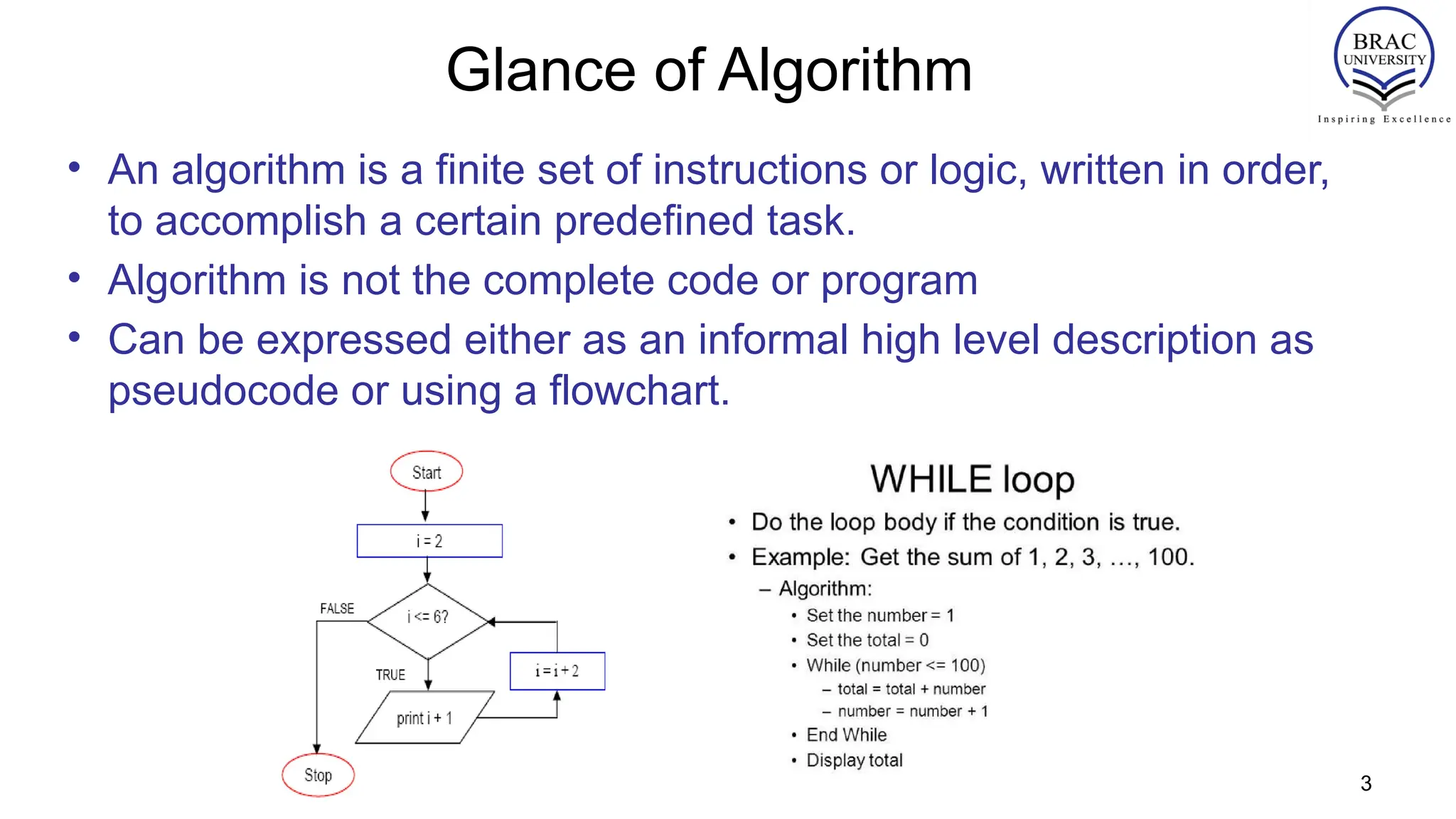
•An algorithm is a finite set of instructions or logic, written in order,
to accomplish a certain predefined task.
• Algorithm is not the complete code or program
• Can be expressed either as an informal high level description as
pseudocode or using a flowchart.
3
4.
Algorithm Specifications
• Input- Every Algorithm must take zero or more number of input values
from external.
• Output - Every Algorithm must produce an output as result.
• Definiteness - Every statement/instruction in an algorithm must be clear
and unambiguous (only one interpretation)
• Finiteness - For all different cases, the algorithm must produce result
within a finite number of steps.
• Effectiveness - Every Instruction must be basic enough to be carried out
and it also must be feasible.
4
5.
Good Algorithms?
• Runin less time
• Consume less memory
But computational resources (time complexity) usually important
5
6.
6
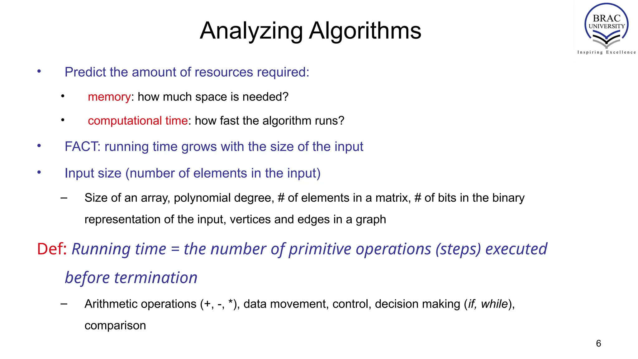
Analyzing Algorithms
• Predictthe amount of resources required:
• memory: how much space is needed?
• computational time: how fast the algorithm runs?
• FACT: running time grows with the size of the input
• Input size (number of elements in the input)
– Size of an array, polynomial degree, # of elements in a matrix, # of bits in the binary
representation of the input, vertices and edges in a graph
Def: Running time = the number of primitive operations (steps) executed
before termination
– Arithmetic operations (+, -, *), data movement, control, decision making (if, while),
comparison
7.
7
Algorithm Analysis: Example
•Alg.: MIN (a[1], …, a[n])
m ← a[1];
for i ← 2 to n
if a[i] < m
then m ← a[i];
• Running time:
– the number of primitive operations (steps) executed before termination
T(n) =1 [first step] + (n) [for loop] + (n-1) [if condition] + (n-1) [the assignment in then] = 3n
- 1
• Order (rate) of growth:
– The leading term of the formula
– Expresses the asymptotic behavior of the algorithm
8.
8
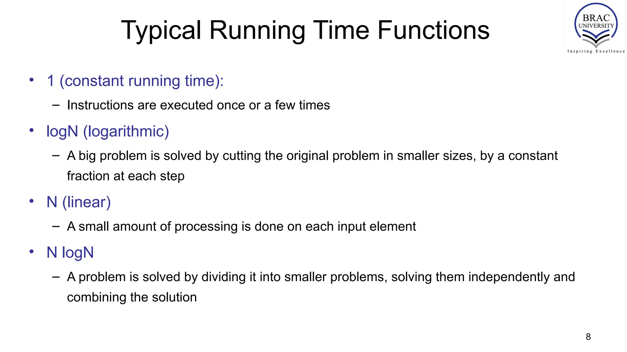
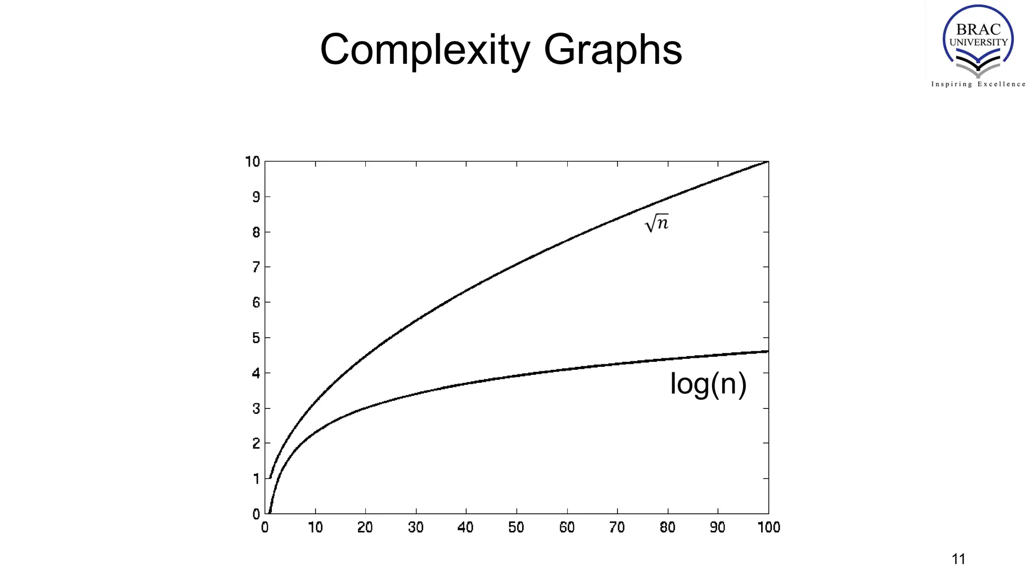
Typical Running TimeFunctions
• 1 (constant running time):
– Instructions are executed once or a few times
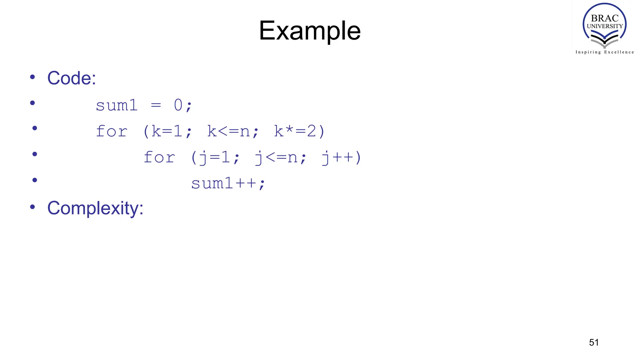
• logN (logarithmic)
– A big problem is solved by cutting the original problem in smaller sizes, by a constant
fraction at each step
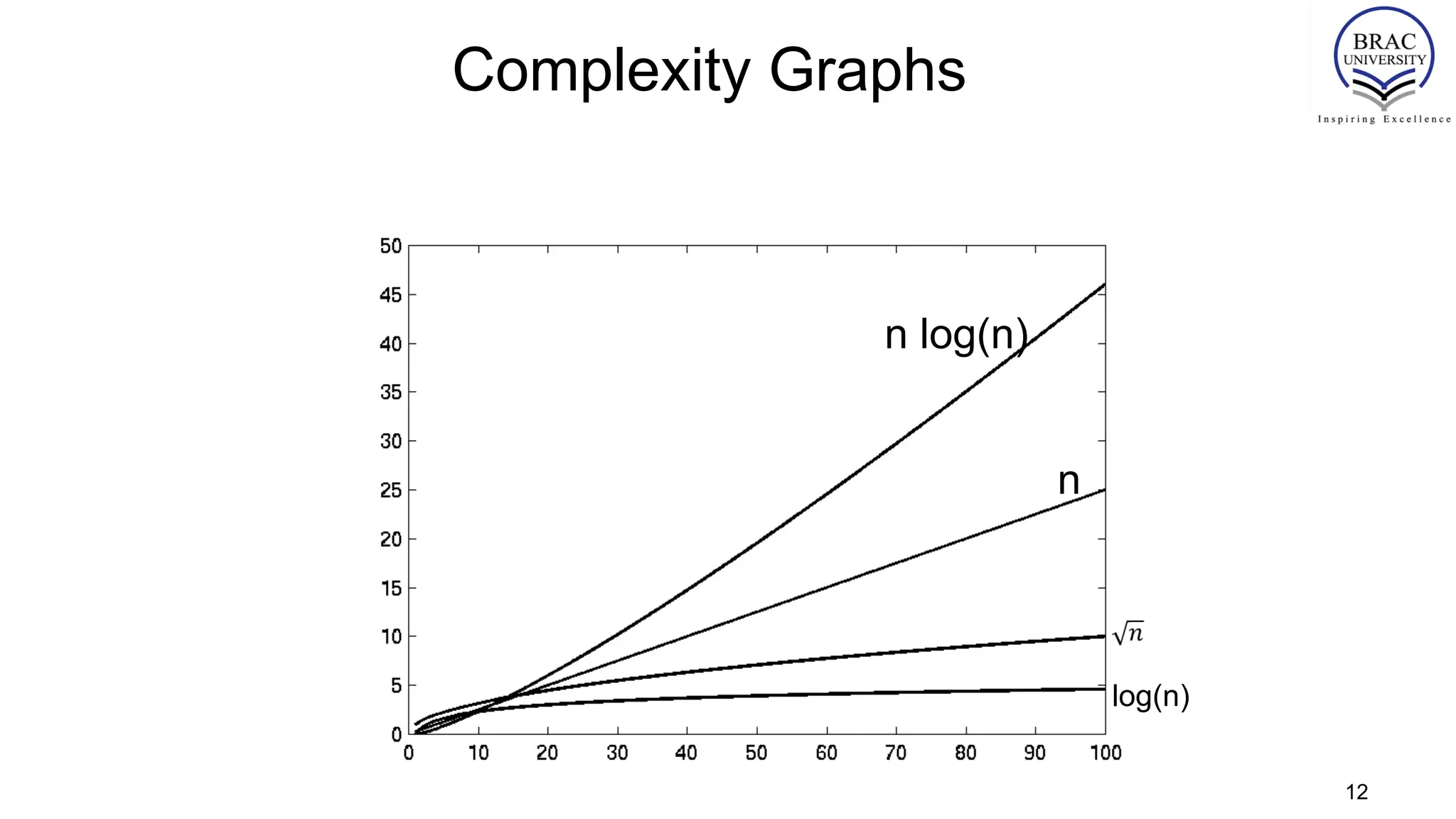
• N (linear)
– A small amount of processing is done on each input element
• N logN
– A problem is solved by dividing it into smaller problems, solving them independently and
combining the solution
9.
9
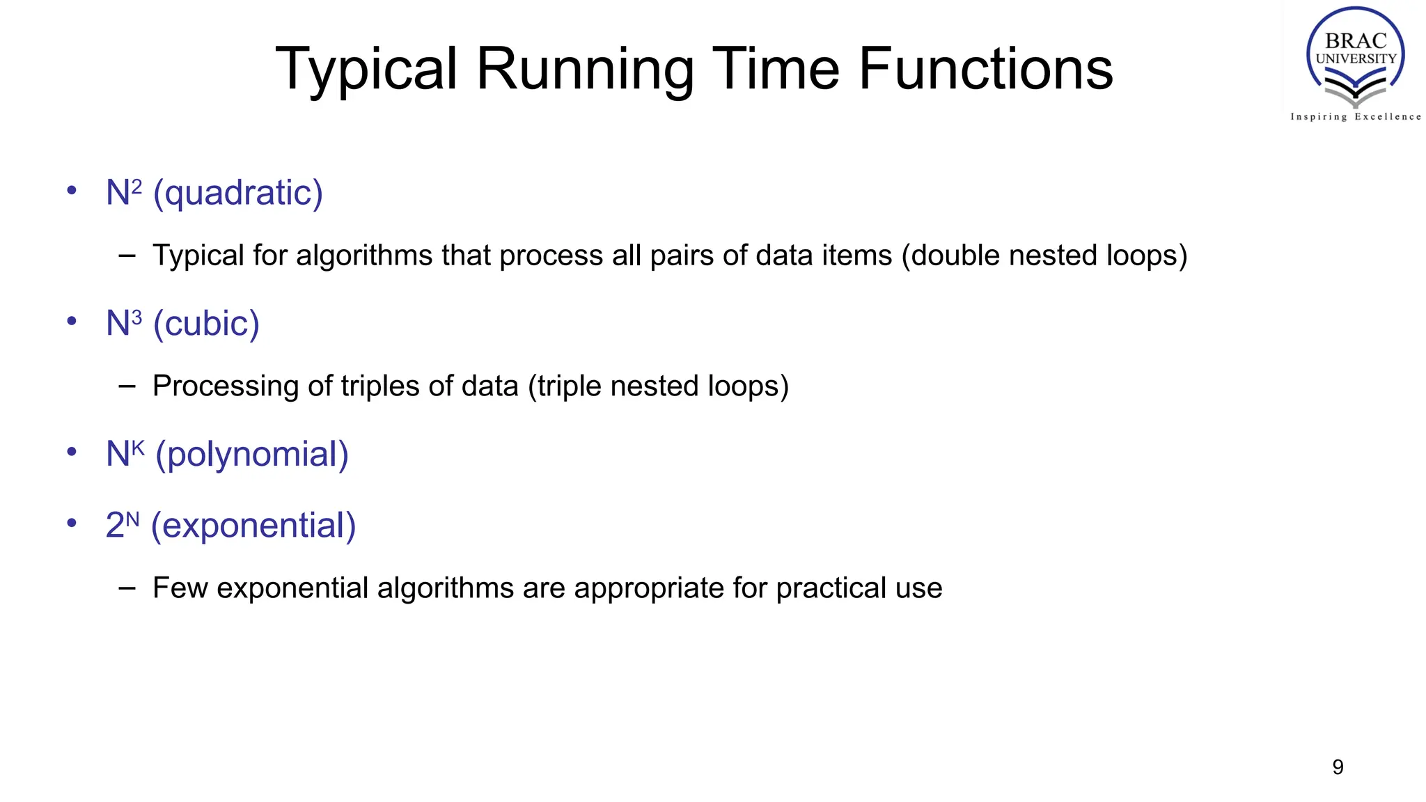
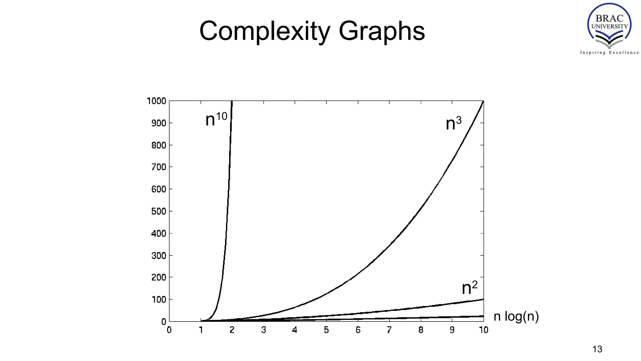
Typical Running TimeFunctions
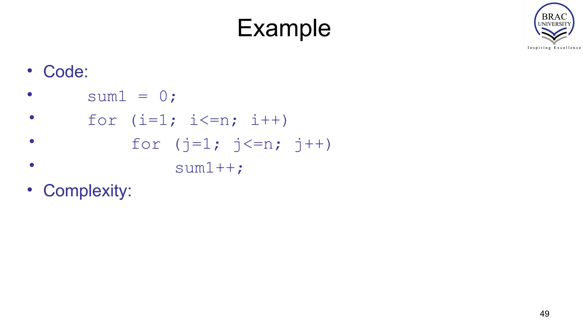
• N2
(quadratic)
– Typical for algorithms that process all pairs of data items (double nested loops)
• N3
(cubic)
– Processing of triples of data (triple nested loops)
• NK
(polynomial)
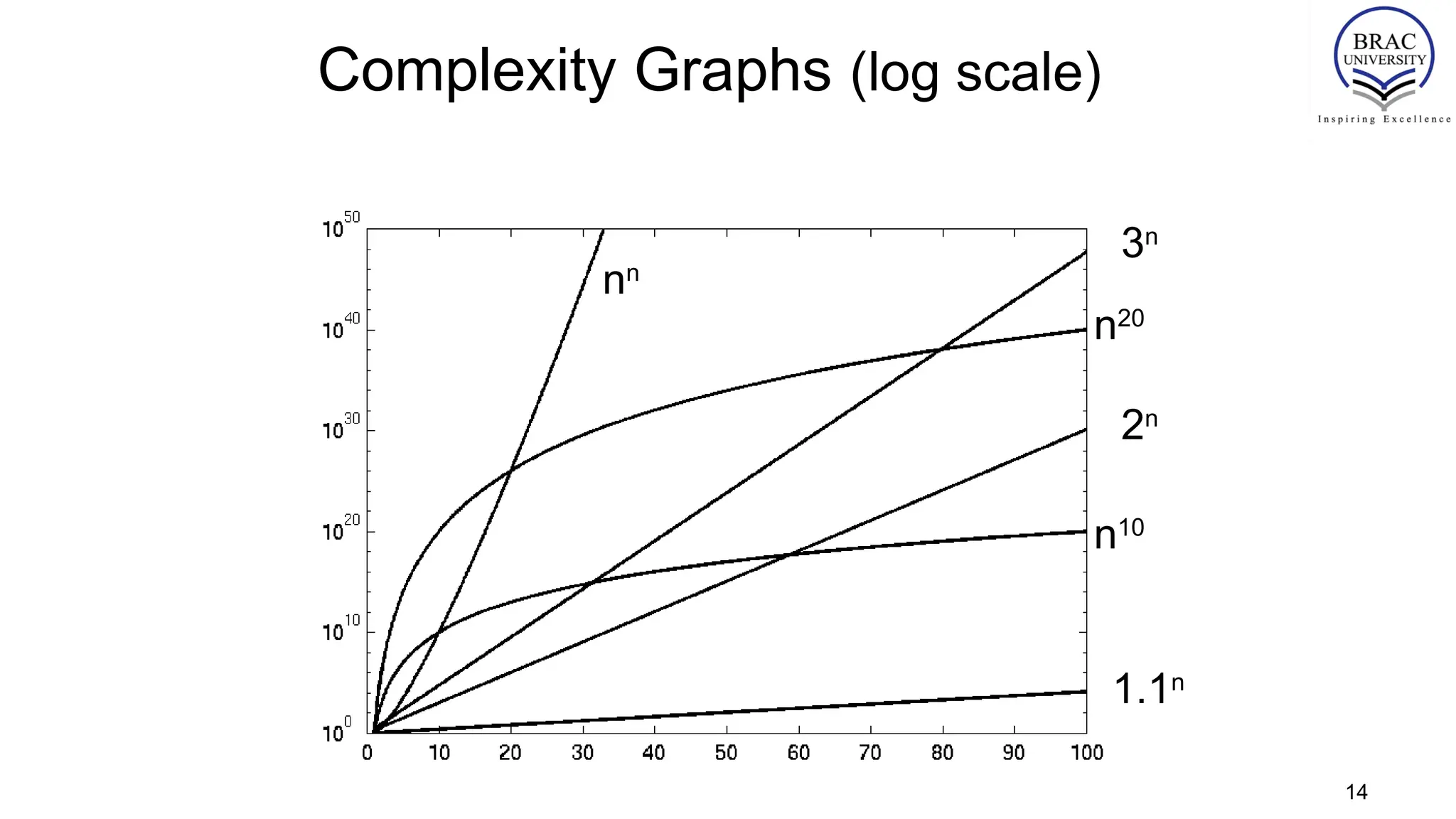
• 2N
(exponential)
– Few exponential algorithms are appropriate for practical use
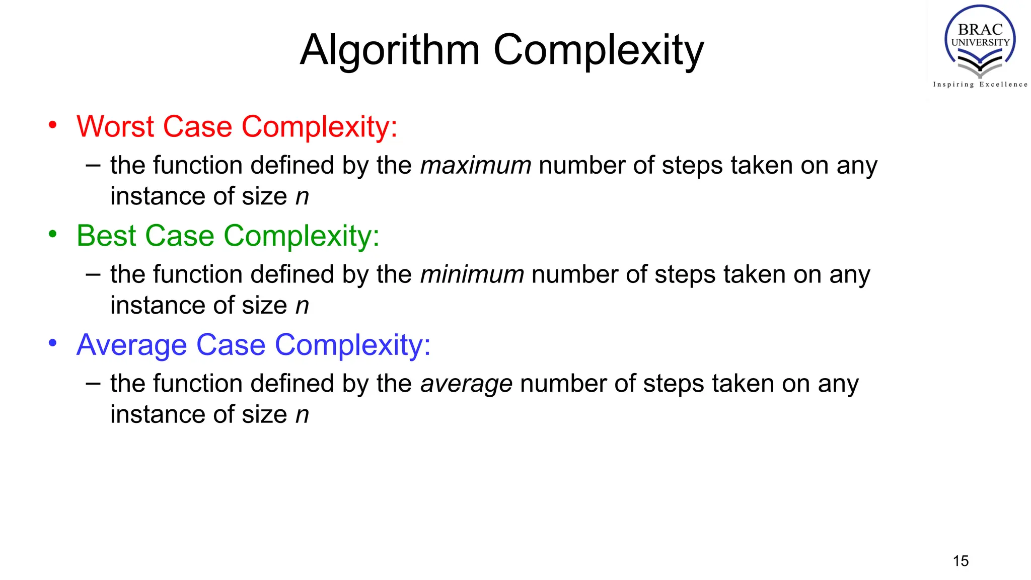
Algorithm Complexity
• WorstCase Complexity:
– the function defined by the maximum number of steps taken on any
instance of size n
• Best Case Complexity:
– the function defined by the minimum number of steps taken on any
instance of size n
• Average Case Complexity:
– the function defined by the average number of steps taken on any
instance of size n
15
16.
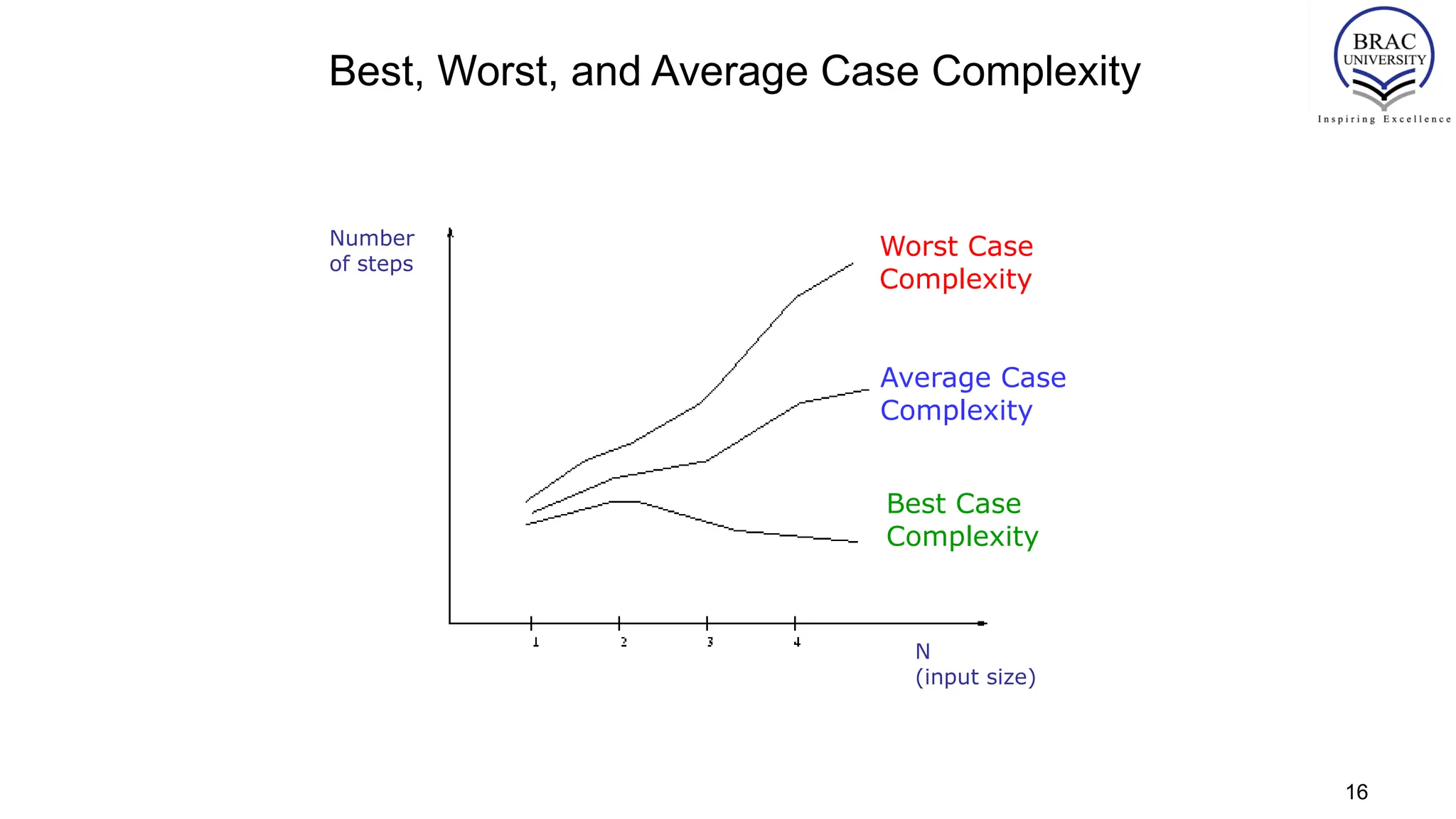
Best, Worst, andAverage Case Complexity
Worst Case
Complexity
Average Case
Complexity
Best Case
Complexity
Number
of steps
N
(input size)
16
17.
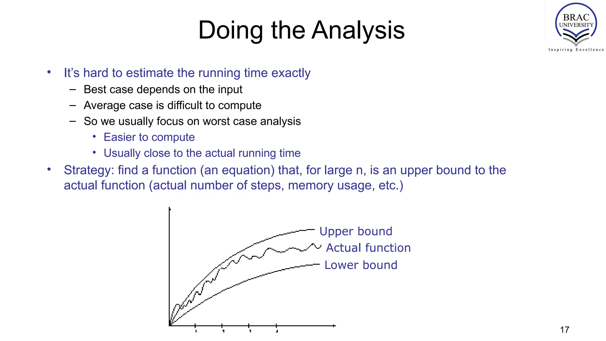
Doing the Analysis
•It’s hard to estimate the running time exactly
– Best case depends on the input
– Average case is difficult to compute
– So we usually focus on worst case analysis
• Easier to compute
• Usually close to the actual running time
• Strategy: find a function (an equation) that, for large n, is an upper bound to the
actual function (actual number of steps, memory usage, etc.)
Upper bound
Lower bound
Actual function
17
18.
Motivation for AsymptoticAnalysis
• An exact computation of worst-case running time can be difficult
– Function may have many terms:
• 4n2
- 3n log n + 17.5 n - 43 n⅔
+ 75
• An exact computation of worst-case running time is unnecessary
18
19.
Classifying functions bytheir
Asymptotic Growth Rates
• asymptotic growth rate, asymptotic order, or
order of functions
– Comparing and classifying functions that ignores
• constant factors and
• small inputs.
• The Sets big oh O(g), big theta Θ(g), big omega Ω(g)
19
20.
Classifying functions bytheir
Asymptotic Growth Rates
1. O(g(n)), Big-Oh of g of n, the Asymptotic Upper Bound
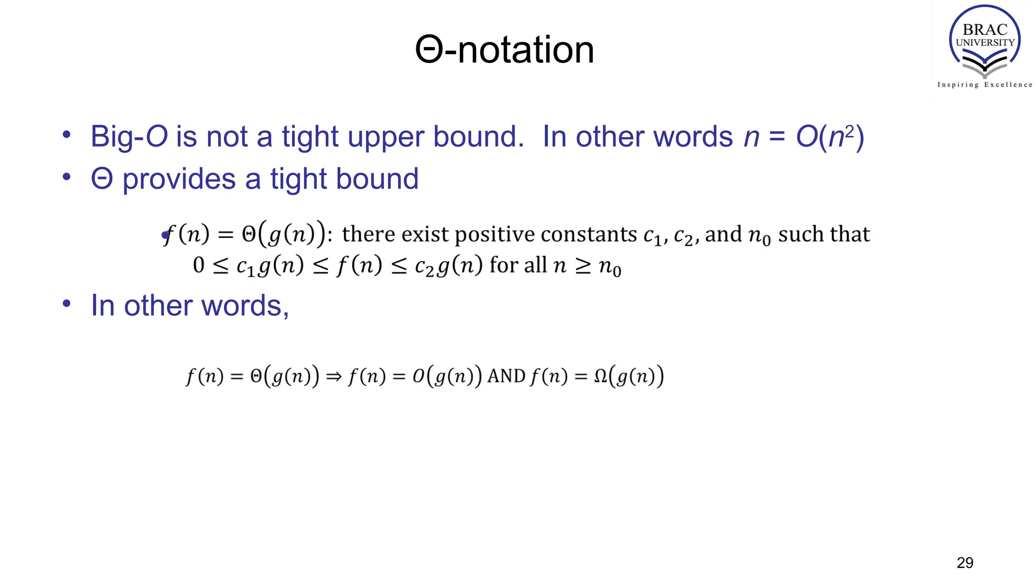
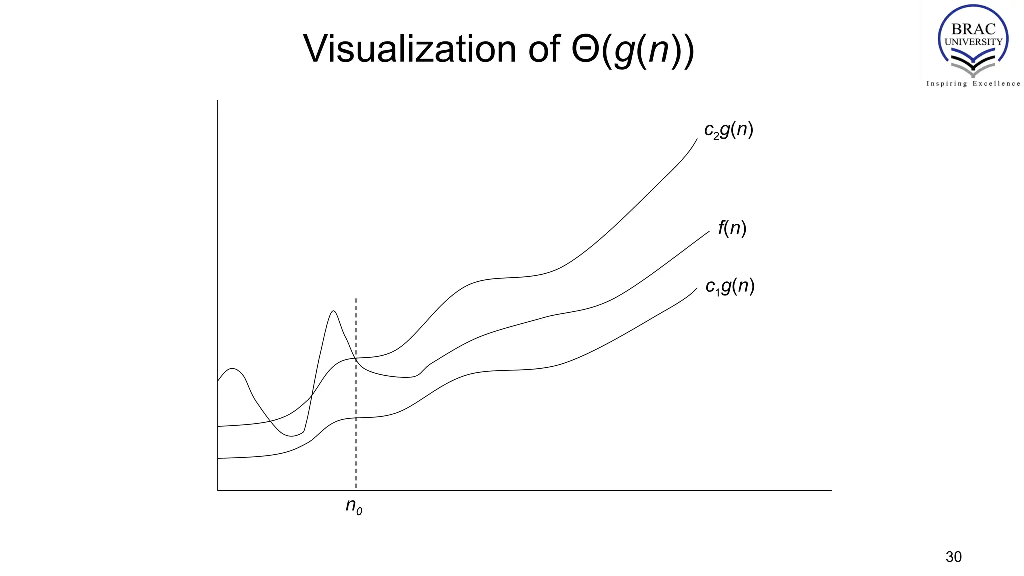
2. Θ(g(n)), Theta of g of n, the Asymptotic Tight Bound
3. Ω(g(n)), Omega of g of n, the Asymptotic Lower Bound
20
21.
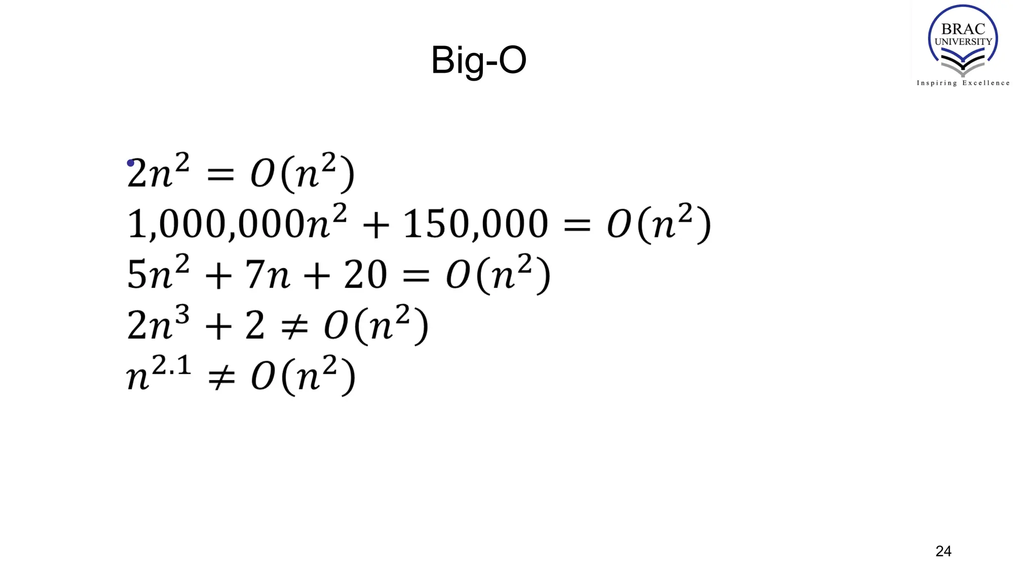
Big-O
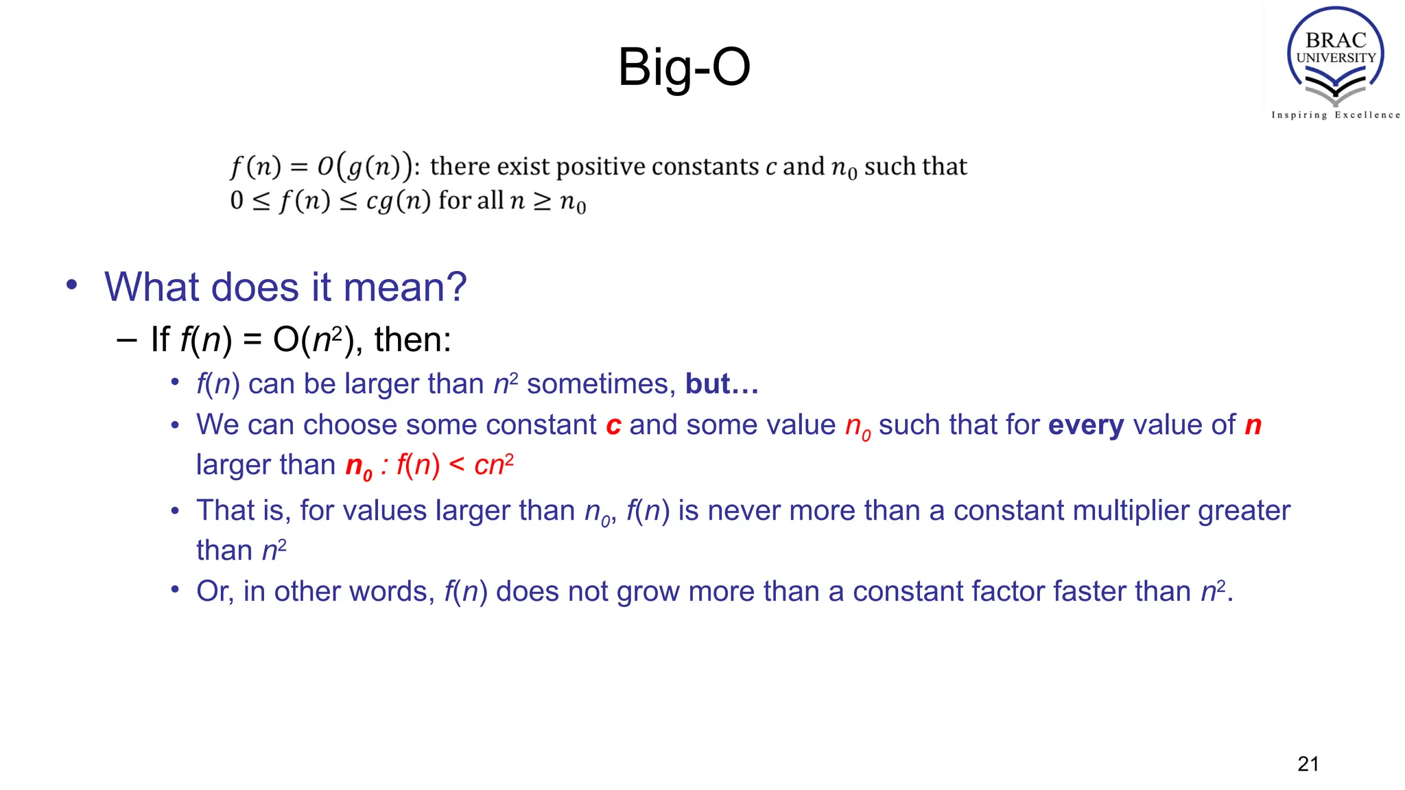
• What doesit mean?
– If f(n) = O(n2
), then:
• f(n) can be larger than n2
sometimes, but…
• We can choose some constant c and some value n0 such that for every value of n
larger than n0 : f(n) < cn2
• That is, for values larger than n0, f(n) is never more than a constant multiplier greater
than n2
• Or, in other words, f(n) does not grow more than a constant factor faster than n2
.
21
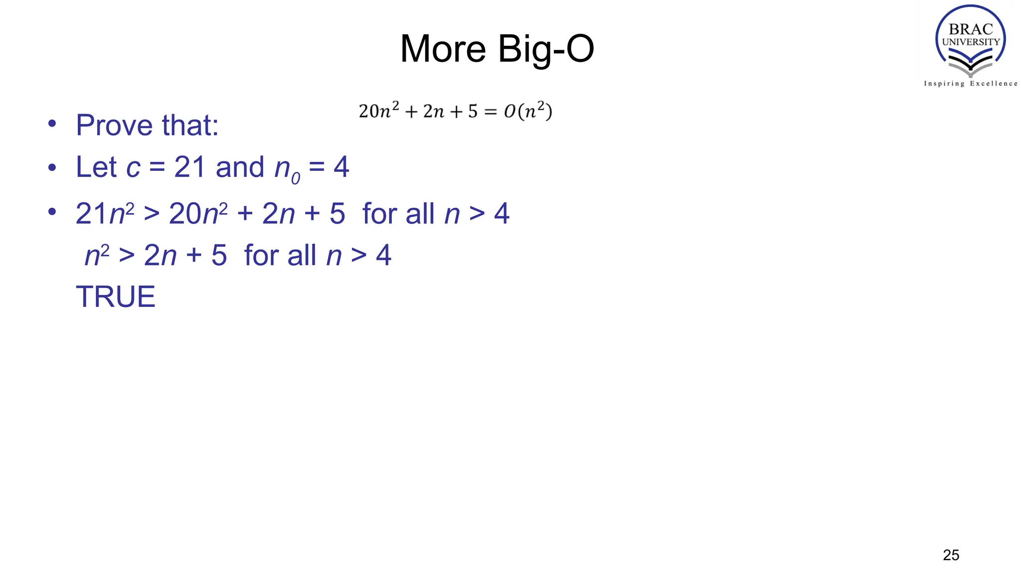
More Big-O
• Provethat:
• Let c = 21 and n0 = 4
• 21n2
> 20n2
+ 2n + 5 for all n > 4
n2
> 2n + 5 for all n > 4
TRUE
25
26.
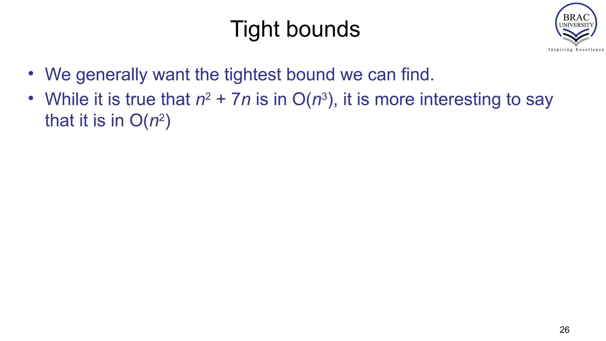
Tight bounds
• Wegenerally want the tightest bound we can find.
• While it is true that n2
+ 7n is in O(n3
), it is more interesting to say
that it is in O(n2
)
26
27.
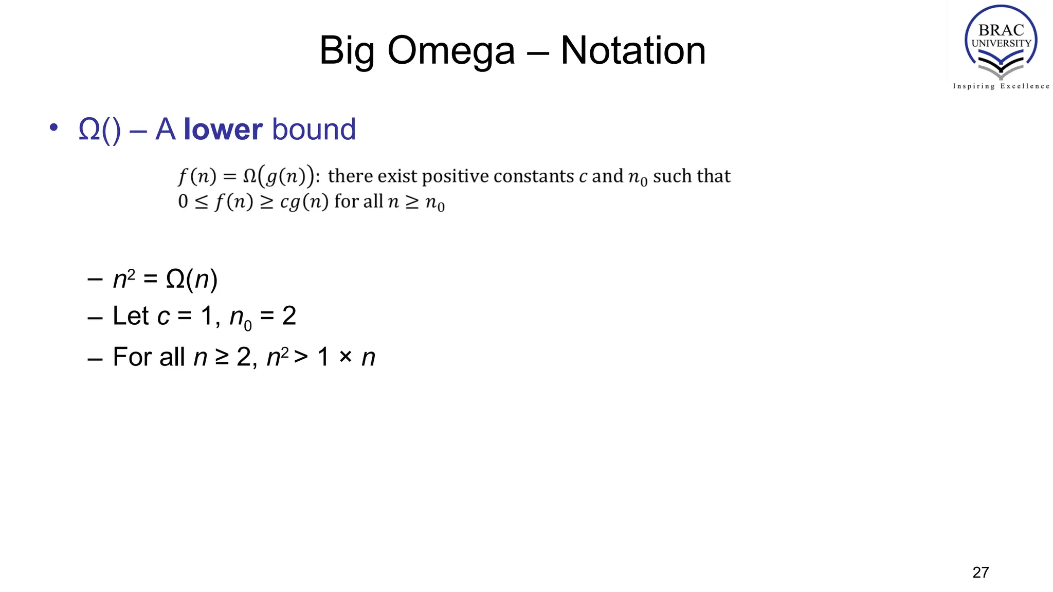
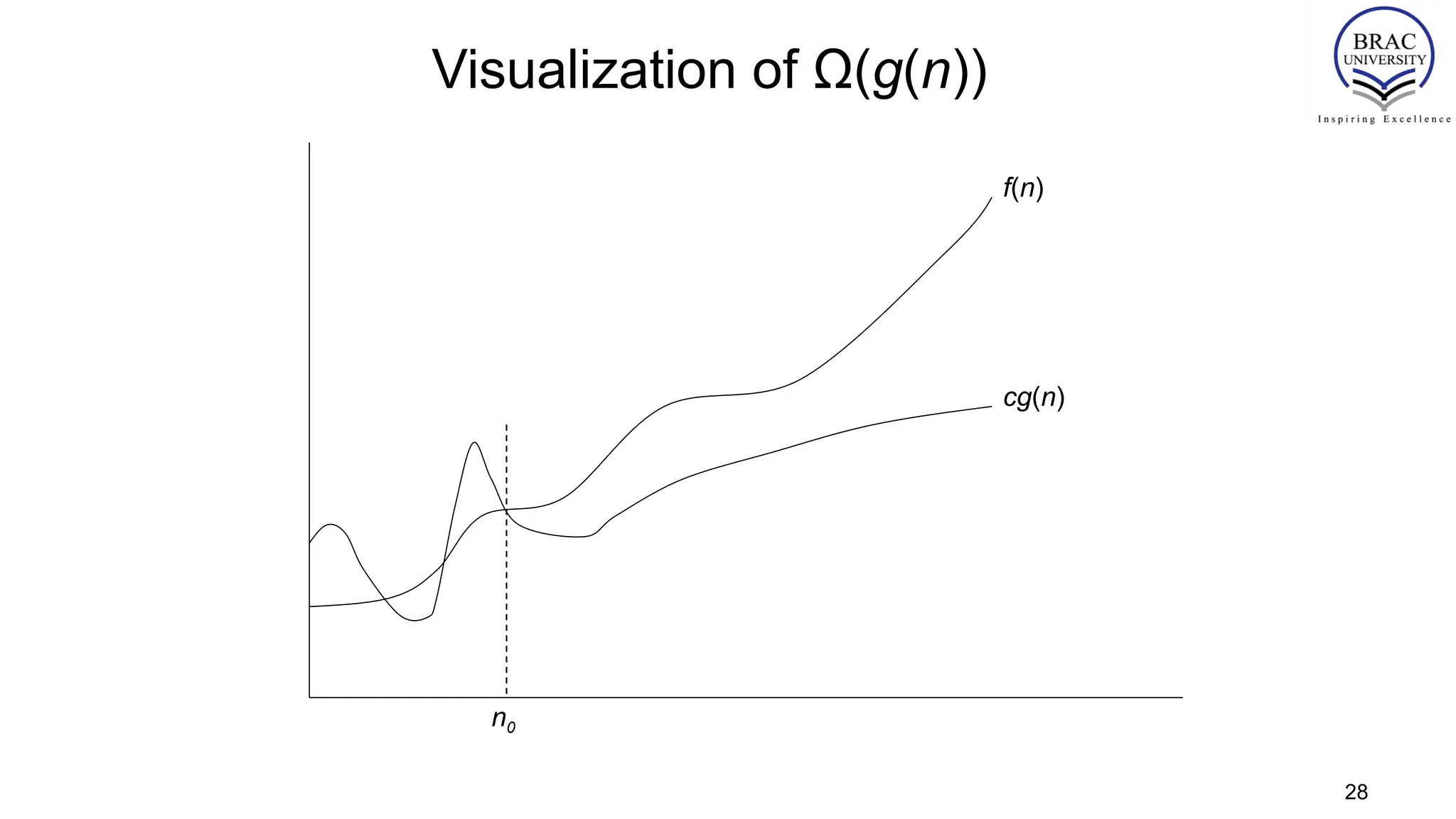
Big Omega –Notation
• Ω() – A lower bound
– n2
= Ω(n)
– Let c = 1, n0 = 2
– For all n ≥ 2, n2
> 1 × n
27
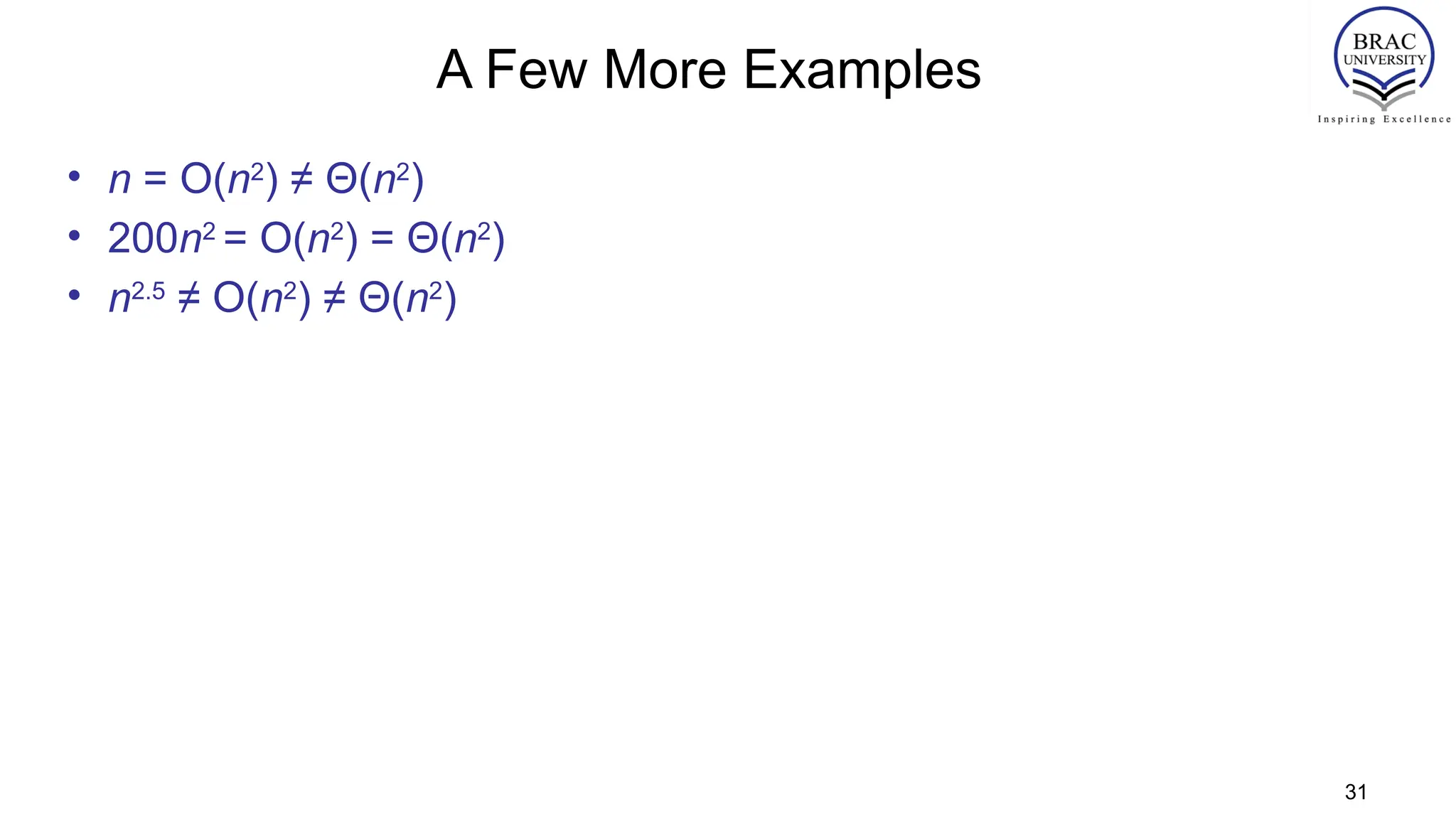
A Few MoreExamples
• n = O(n2
) ≠ Θ(n2
)
• 200n2
= O(n2
) = Θ(n2
)
• n2.5
≠ O(n2
) ≠ Θ(n2
)
31
32.
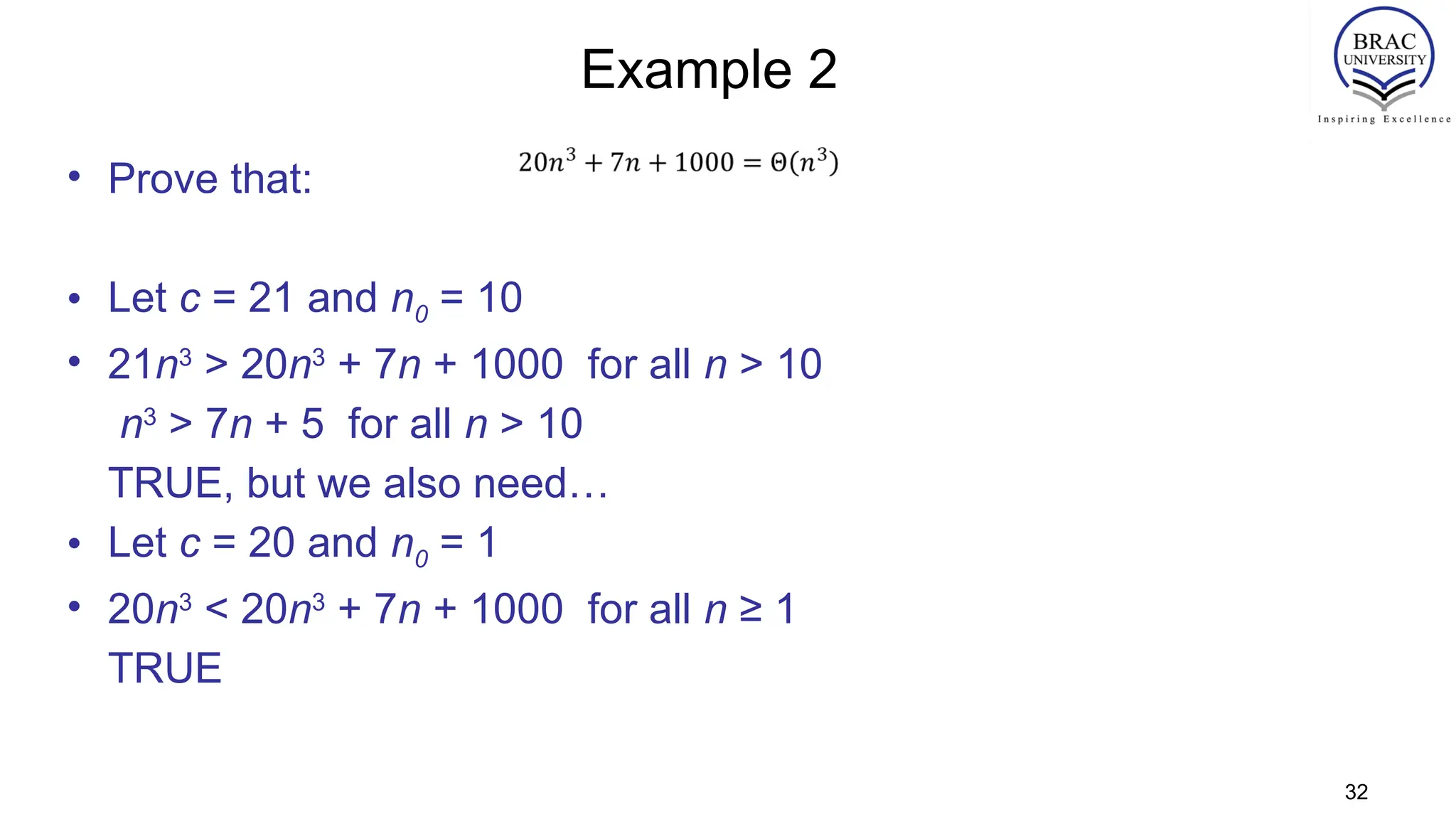
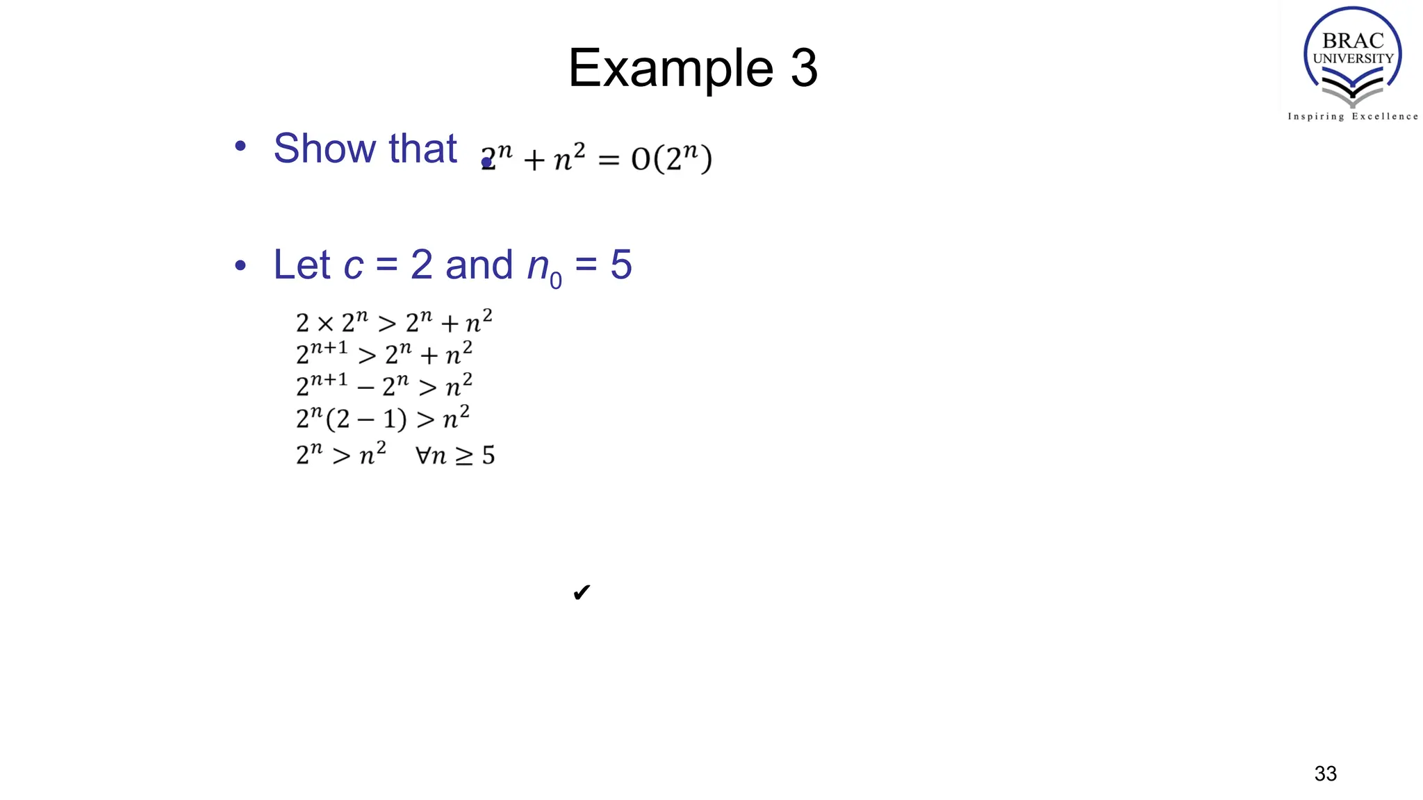
Example 2
• Provethat:
• Let c = 21 and n0 = 10
• 21n3
> 20n3
+ 7n + 1000 for all n > 10
n3
> 7n + 5 for all n > 10
TRUE, but we also need…
• Let c = 20 and n0 = 1
• 20n3
< 20n3
+ 7n + 1000 for all n ≥ 1
TRUE
32
34
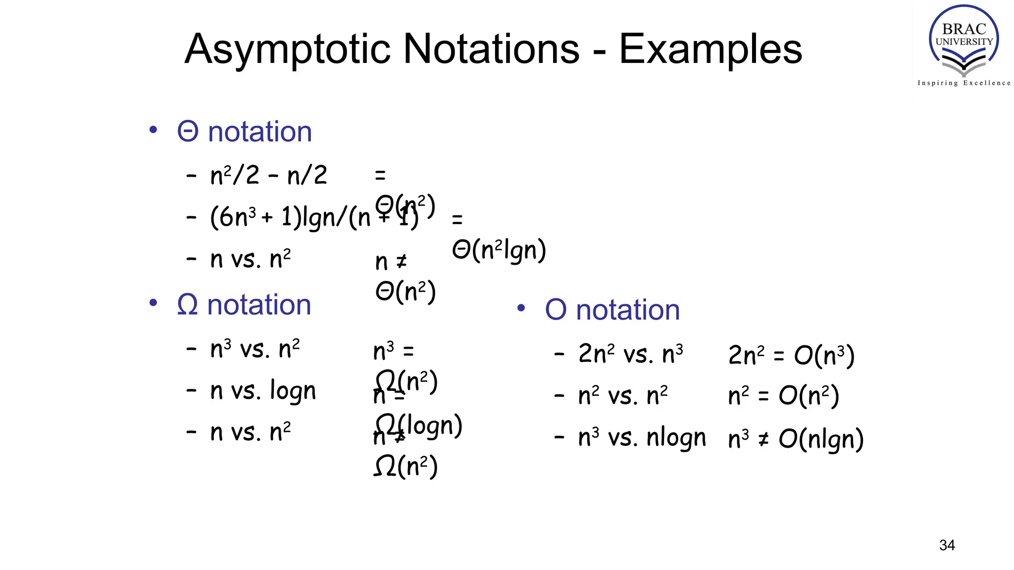
Asymptotic Notations -Examples
• Θ notation
– n2
/2 – n/2
– (6n3
+ 1)lgn/(n + 1)
– n vs. n2
• Ω notation
– n3
vs. n2
– n vs. logn
– n vs. n2
=
Θ(n2
)
n ≠
Θ(n2
)
=
Θ(n2
lgn)
• O notation
– 2n2
vs. n3
– n2
vs. n2
– n3
vs. nlogn
n3
=
Ω(n2
)
n =
Ω(logn)
n ≠
Ω(n2
)
2n2
= O(n3
)
n2
= O(n2
)
n3
≠ O(nlgn)
35.
35
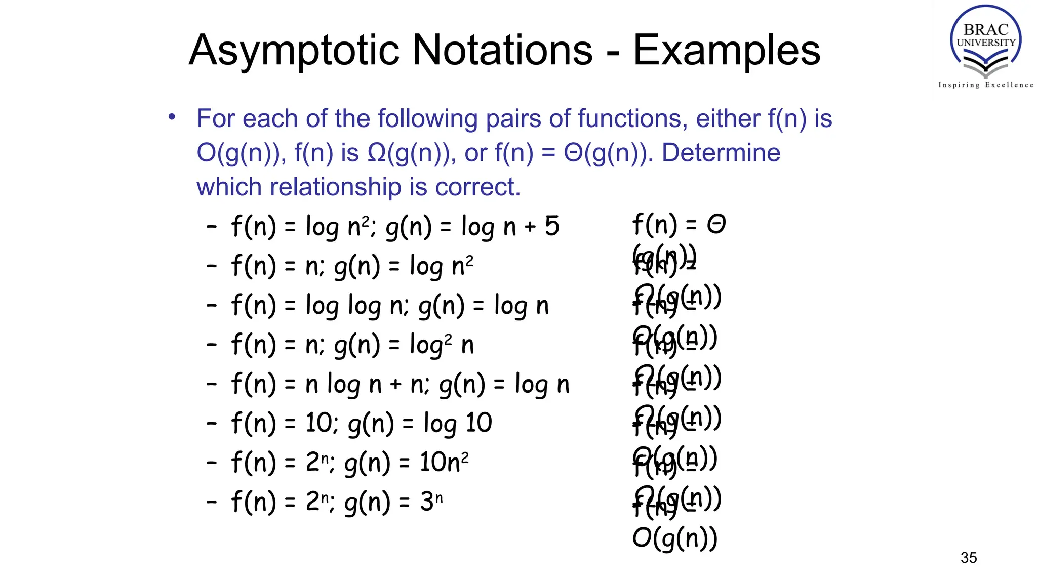
Asymptotic Notations -Examples
• For each of the following pairs of functions, either f(n) is
O(g(n)), f(n) is Ω(g(n)), or f(n) = Θ(g(n)). Determine
which relationship is correct.
– f(n) = log n2
; g(n) = log n + 5
– f(n) = n; g(n) = log n2
– f(n) = log log n; g(n) = log n
– f(n) = n; g(n) = log2
n
– f(n) = n log n + n; g(n) = log n
– f(n) = 10; g(n) = log 10
– f(n) = 2n
; g(n) = 10n2
– f(n) = 2n
; g(n) = 3n
f(n) = Θ
(g(n))
f(n) =
Ω(g(n))
f(n) =
O(g(n))
f(n) =
Ω(g(n))
f(n) =
Ω(g(n))
f(n) =
Θ(g(n))
f(n) =
Ω(g(n))
f(n) =
O(g(n))
36.
36
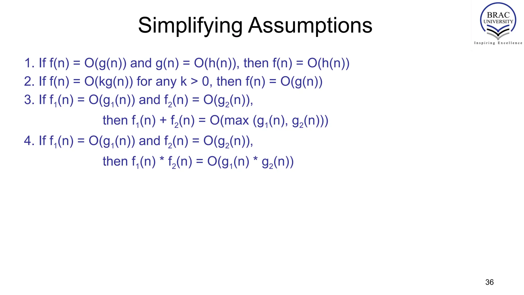
Simplifying Assumptions
1. Iff(n) = O(g(n)) and g(n) = O(h(n)), then f(n) = O(h(n))
2. If f(n) = O(kg(n)) for any k > 0, then f(n) = O(g(n))
3. If f1(n) = O(g1(n)) and f2(n) = O(g2(n)),
then f1(n) + f2(n) = O(max (g1(n), g2(n)))
4. If f1(n) = O(g1(n)) and f2(n) = O(g2(n)),
then f1(n) * f2(n) = O(g1(n) * g2(n))
37.
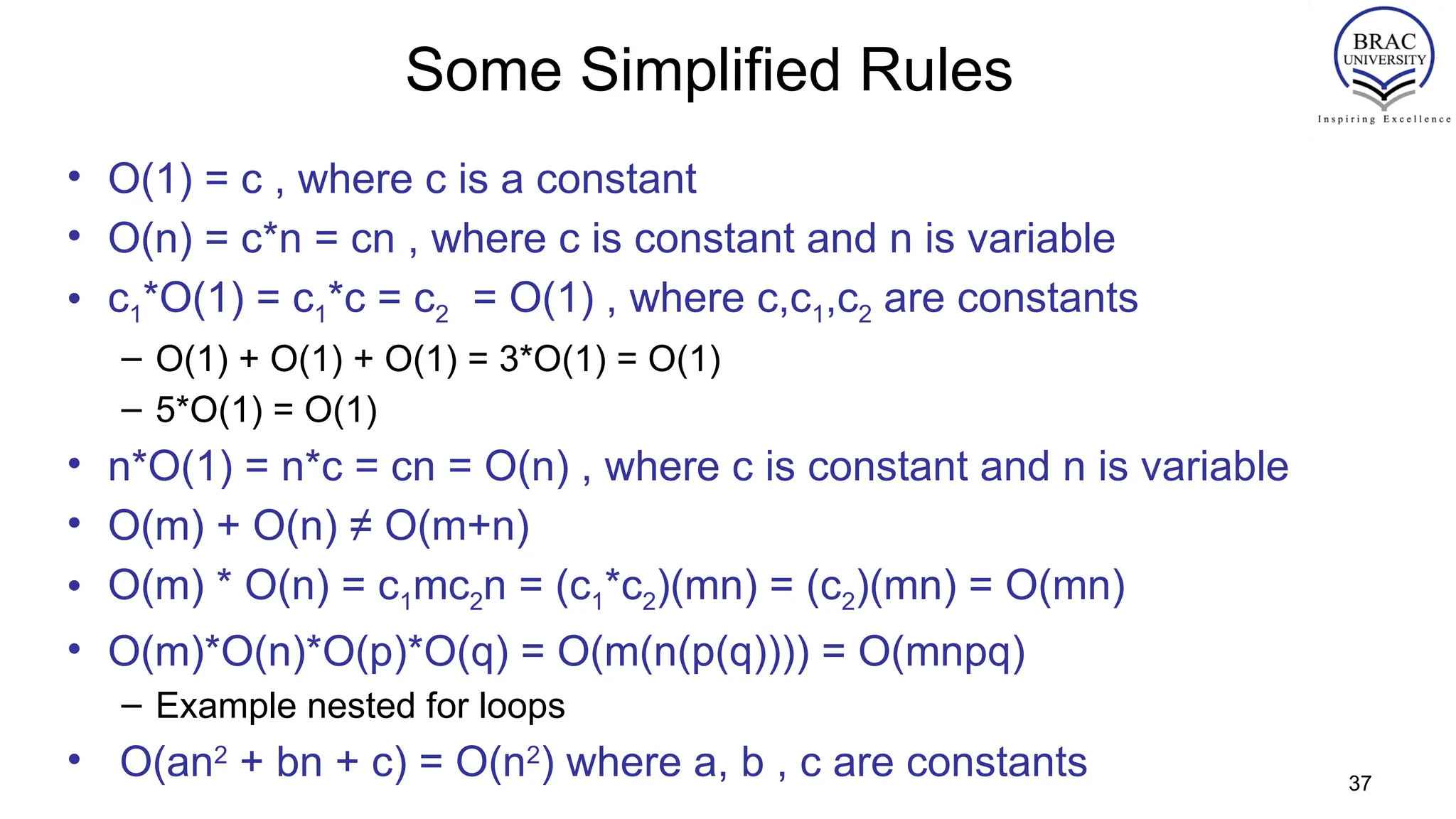
Some Simplified Rules
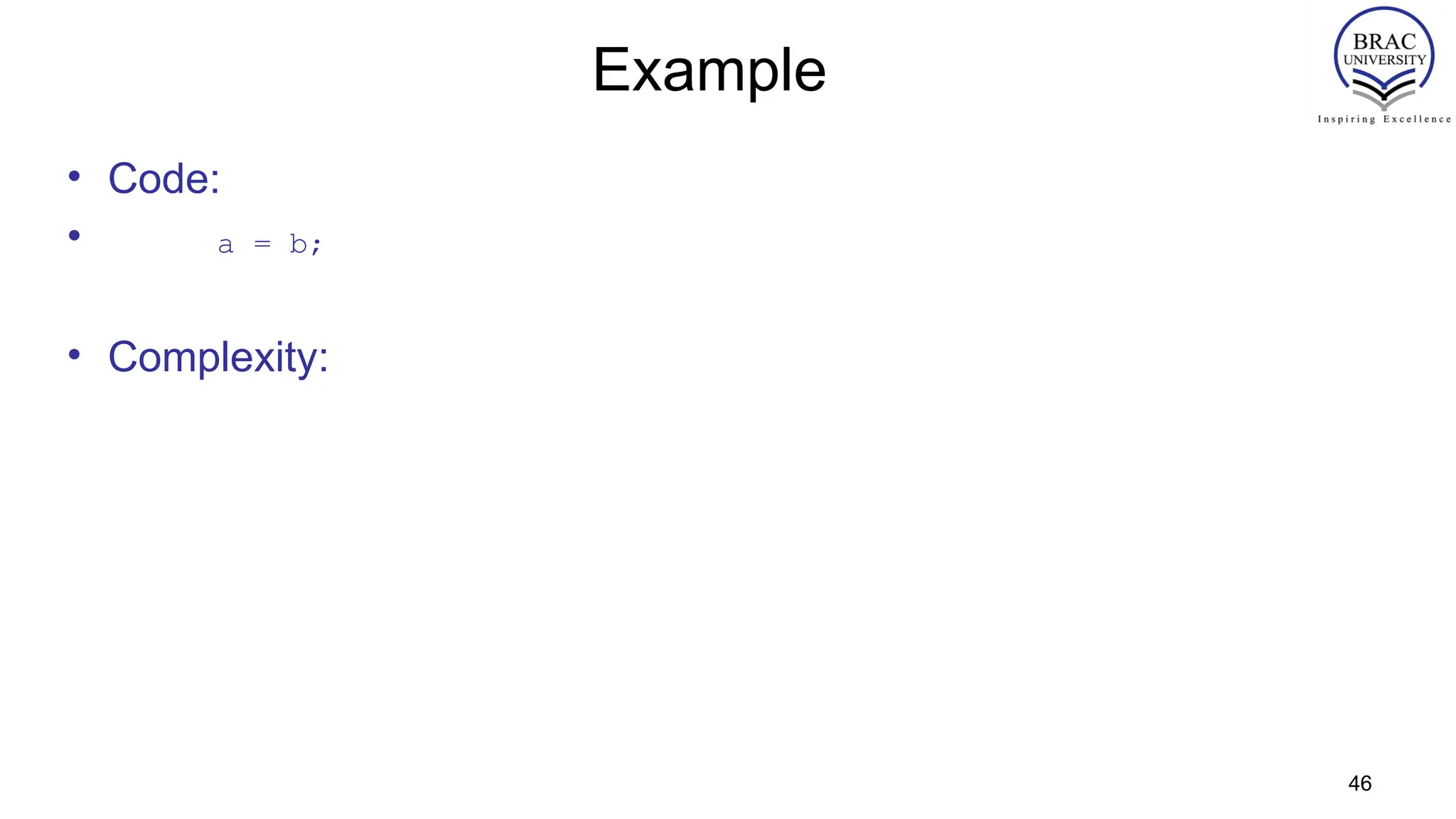
•O(1) = c , where c is a constant
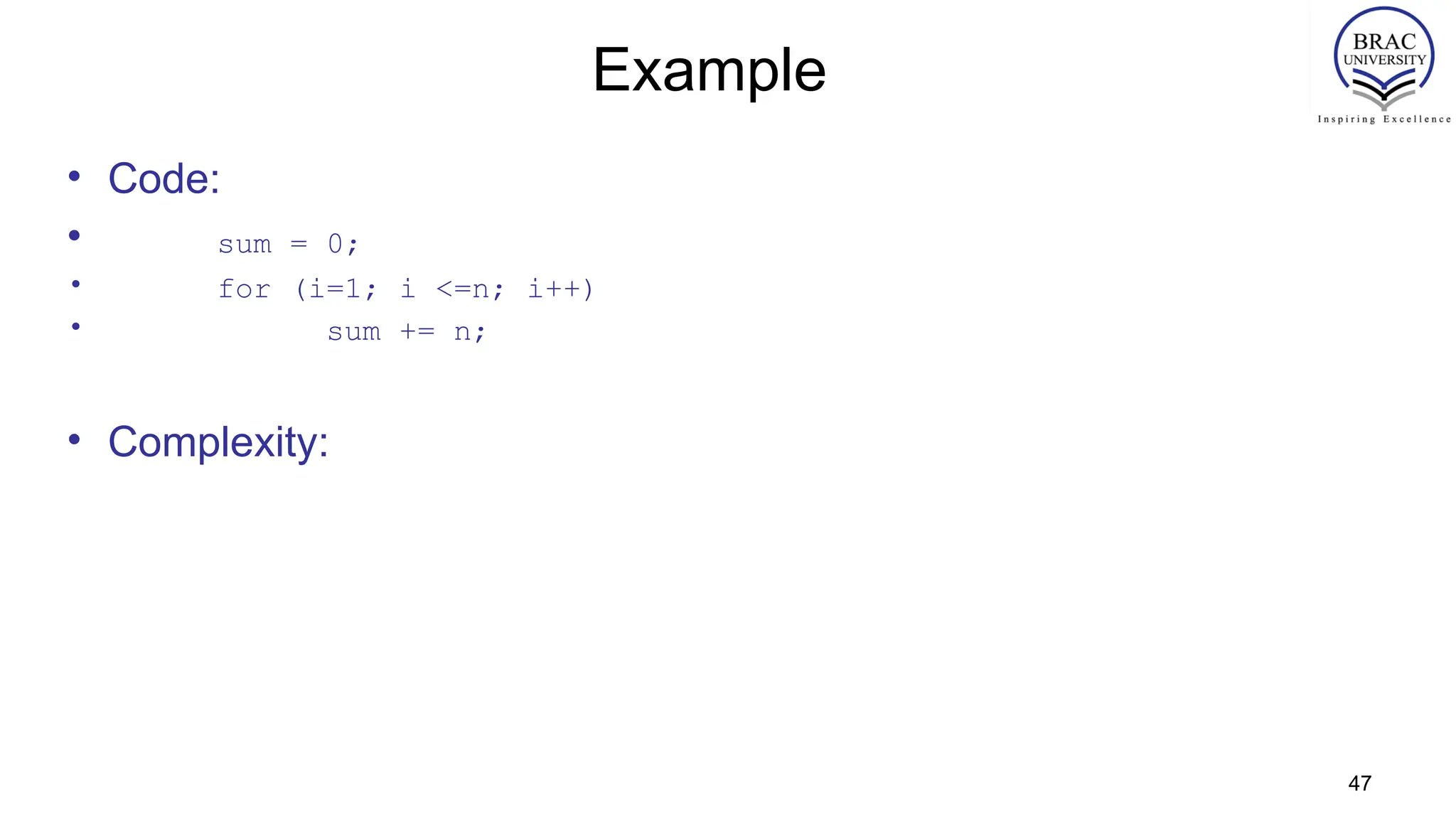
• O(n) = c*n = cn , where c is constant and n is variable
• c1*O(1) = c1*c = c2 = O(1) , where c,c1,c2 are constants
– O(1) + O(1) + O(1) = 3*O(1) = O(1)
– 5*O(1) = O(1)
• n*O(1) = n*c = cn = O(n) , where c is constant and n is variable
• O(m) + O(n) ≠ O(m+n)
• O(m) * O(n) = c1mc2n = (c1*c2)(mn) = (c2)(mn) = O(mn)
• O(m)*O(n)*O(p)*O(q) = O(m(n(p(q)))) = O(mnpq)
– Example nested for loops
• O(an2
+ bn + c) = O(n2
) where a, b , c are constants 37
38.
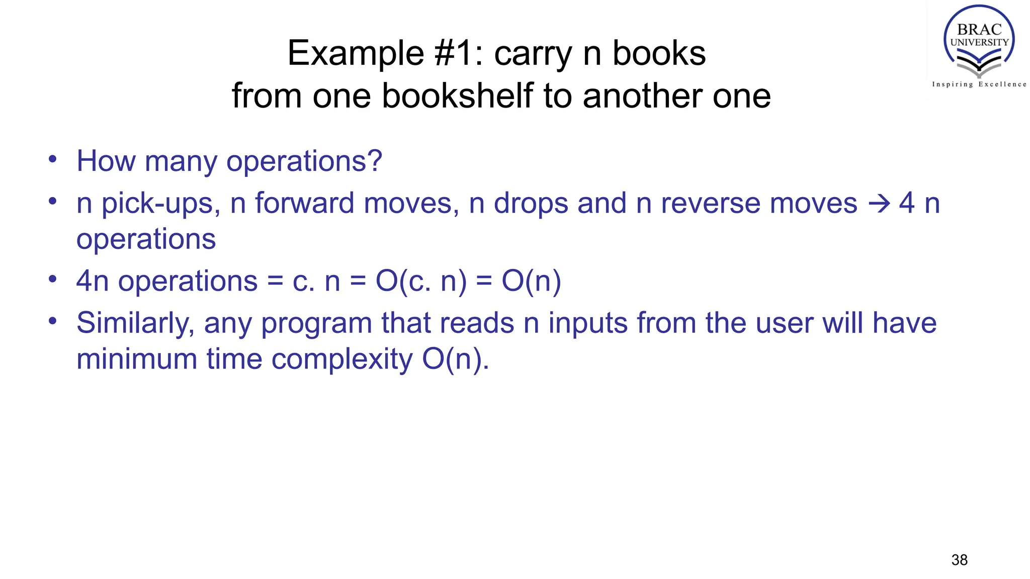
Example #1: carryn books
from one bookshelf to another one
• How many operations?
• n pick-ups, n forward moves, n drops and n reverse moves 4 n
🡪
operations
• 4n operations = c. n = O(c. n) = O(n)
• Similarly, any program that reads n inputs from the user will have
minimum time complexity O(n).
38
39.
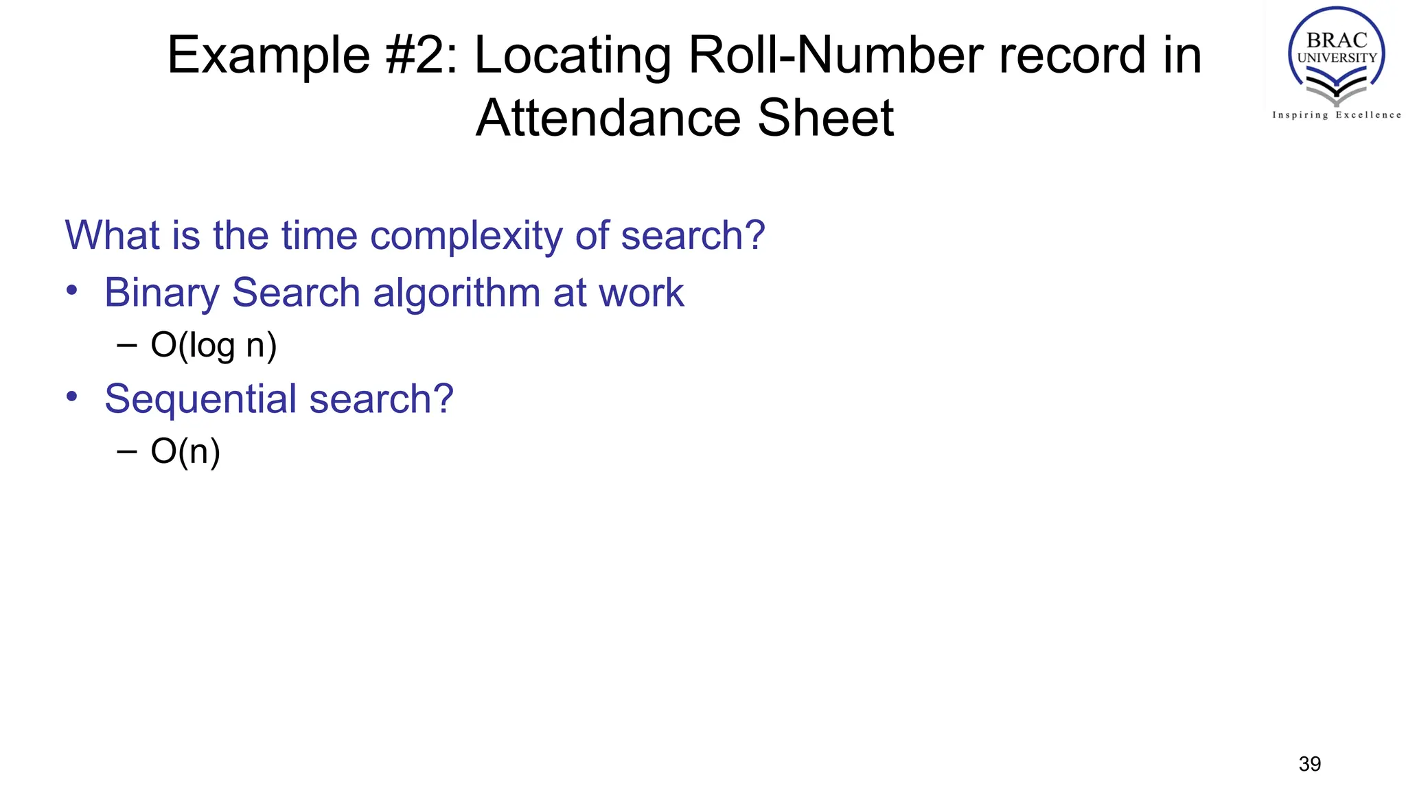
Example #2: LocatingRoll-Number record in
Attendance Sheet
What is the time complexity of search?
• Binary Search algorithm at work
– O(log n)
• Sequential search?
– O(n)
39
40.
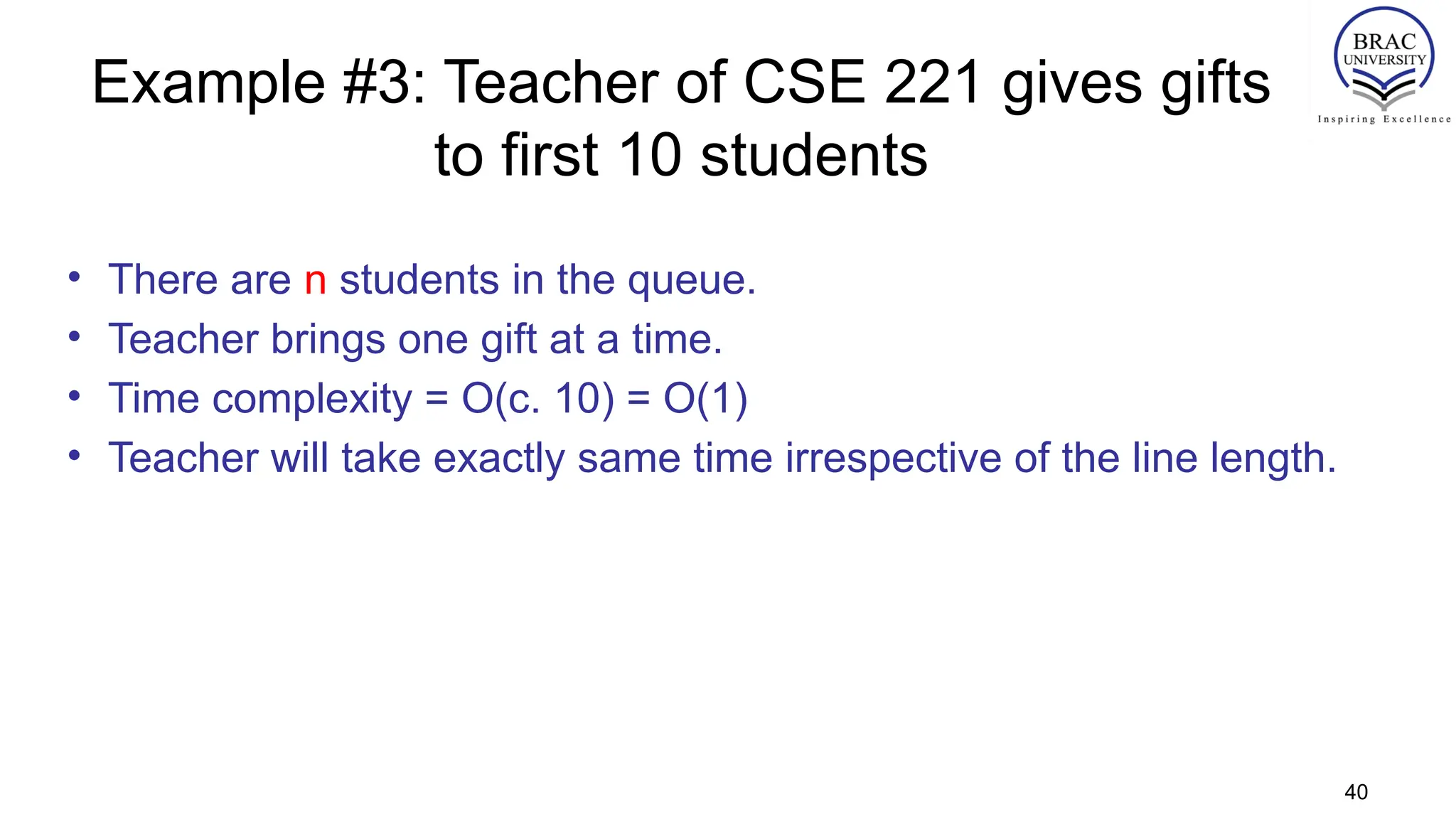
Example #3: Teacherof CSE 221 gives gifts
to first 10 students
• There are n students in the queue.
• Teacher brings one gift at a time.
• Time complexity = O(c. 10) = O(1)
• Teacher will take exactly same time irrespective of the line length.
40
41.
41
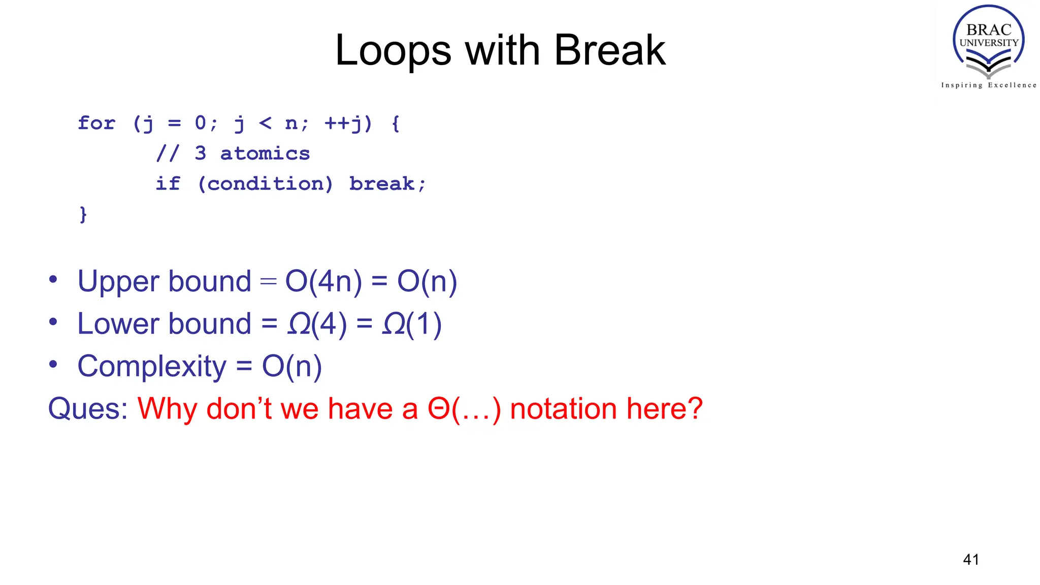
Loops with Break
for(j = 0; j < n; ++j) {
// 3 atomics
if (condition) break;
}
• Upper bound = O(4n) = O(n)
• Lower bound = Ω(4) = Ω(1)
• Complexity = O(n)
Ques: Why don’t we have a Θ(…) notation here?
42.
42
Sequential Search
• Givenan unsorted vector/list a[ ], find the location of element X.
for (i = 0; i < n; i++) {
if (a[i] == X) return true;
}
return false;
• Input size: n = array size()
• Complexity = O(n)
54
Binary Search
• Givena sorted vector/list a[ ], find the location of element X
unsigned int binary_search(vector<int> a, int X)
{
unsigned int low = 0, high = a.size()-1;
while (low <= high) {
int mid = (low + high) / 2;
if (a[mid] < X)
low = mid + 1;
else if( a[mid] > X )
high = mid - 1;
else
return mid;
}
return NOT_FOUND;
}
• Input size: n = array size()
• Complexity = O( k iterations x (1 comparison+1 assignment) per loop)
= O(log(n))
55.
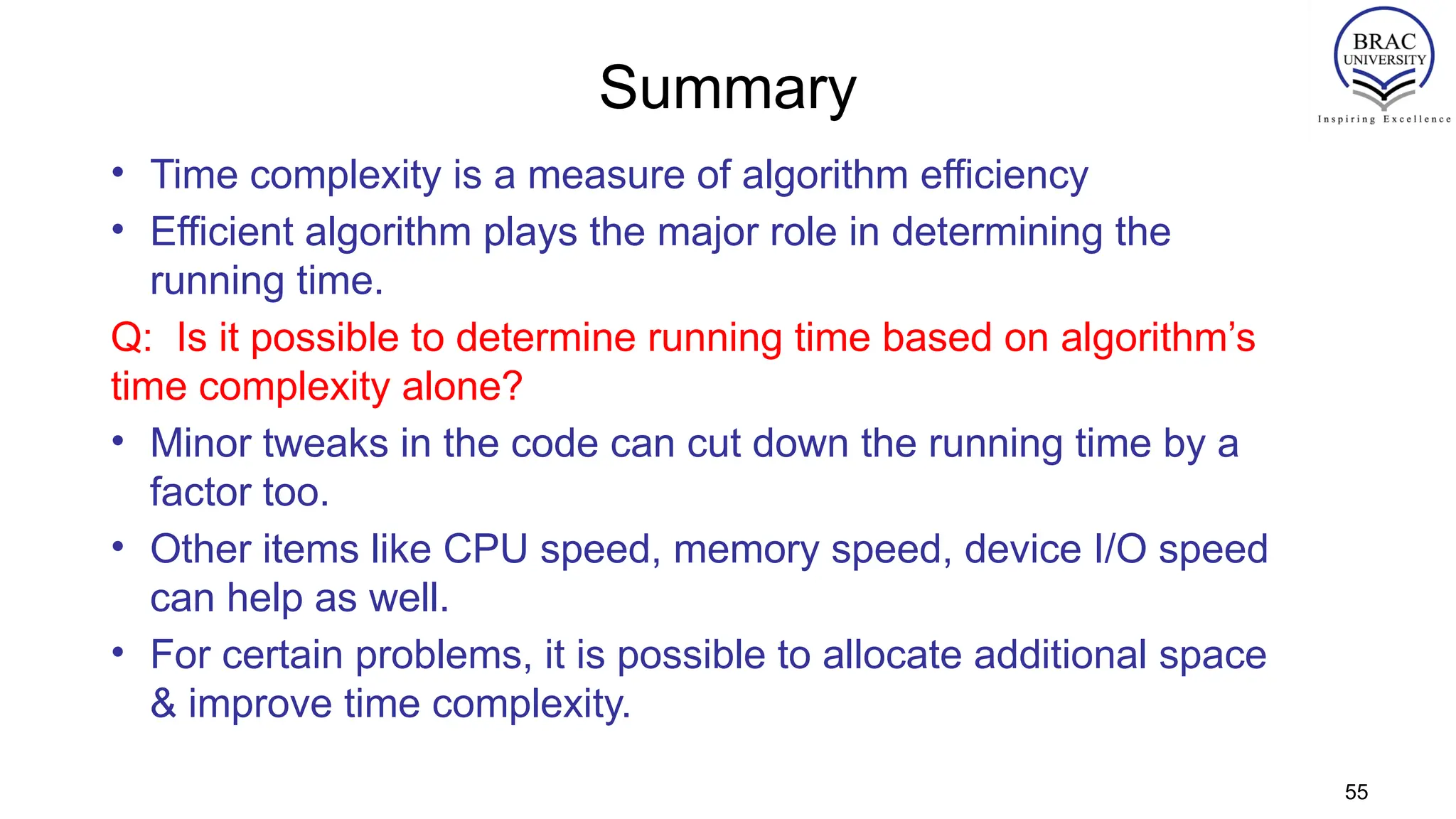
Summary
• Time complexityis a measure of algorithm efficiency
• Efficient algorithm plays the major role in determining the
running time.
Q: Is it possible to determine running time based on algorithm’s
time complexity alone?
• Minor tweaks in the code can cut down the running time by a
factor too.
• Other items like CPU speed, memory speed, device I/O speed
can help as well.
• For certain problems, it is possible to allocate additional space
& improve time complexity.
55
56.
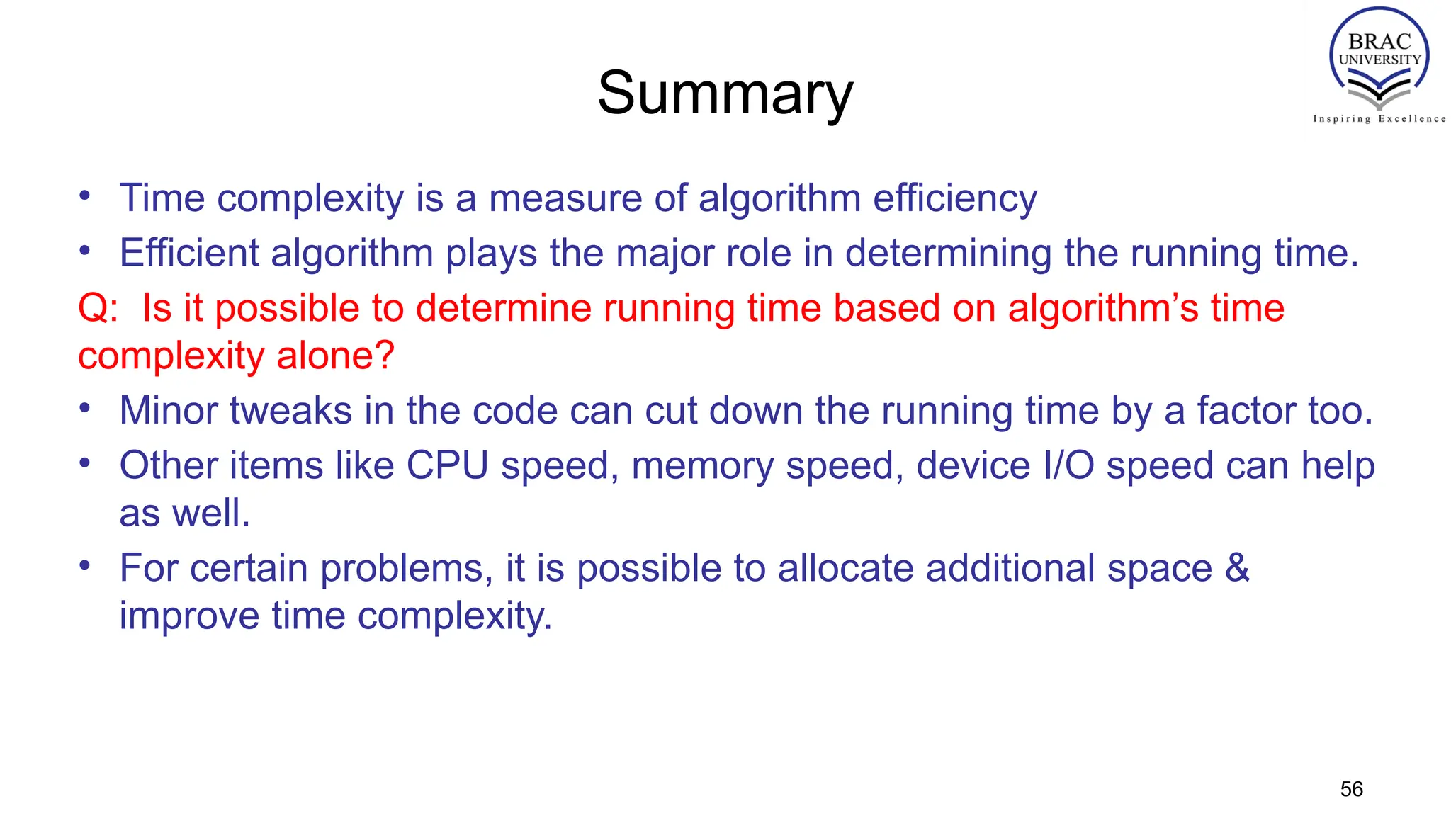
Summary
• Time complexityis a measure of algorithm efficiency
• Efficient algorithm plays the major role in determining the running time.
Q: Is it possible to determine running time based on algorithm’s time
complexity alone?
• Minor tweaks in the code can cut down the running time by a factor too.
• Other items like CPU speed, memory speed, device I/O speed can help
as well.
• For certain problems, it is possible to allocate additional space &
improve time complexity.
56
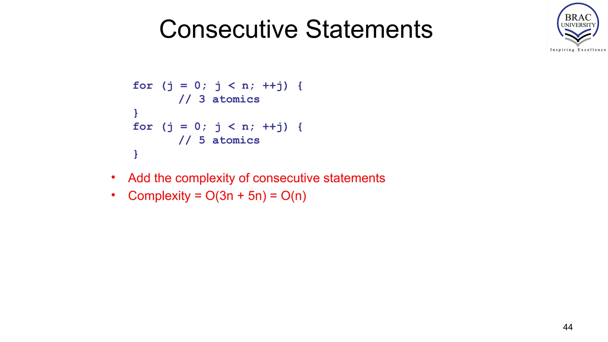
Editor's Notes
#18 Random Access Machine (RAM) model. This model assumes a single processor. In the RAM model, instructions are executed one after the other, with no concurrent operations. This model of computation is an abstraction that allows us to compare algorithms on the basis of performance. The assumptions made in the RAM model to accomplish this are:
Each simple operation takes 1 time step.
Loops and subroutines are not simple operations.
Each memory access takes one time step, and there is no shortage of memory.
#20 asymptotically tight bound: Definition: When the asymptotic complexity of an algorithm exactly matches the theoretically proved asymptotic complexity of the corresponding problem. Informally, when an algorithm solves a problem at the theoretical minimum.
![7
Algorithm Analysis: Example
• Alg.: MIN (a[1], …, a[n])
m ← a[1];
for i ← 2 to n
if a[i] < m
then m ← a[i];
• Running time:
– the number of primitive operations (steps) executed before termination
T(n) =1 [first step] + (n) [for loop] + (n-1) [if condition] + (n-1) [the assignment in then] = 3n
- 1
• Order (rate) of growth:
– The leading term of the formula
– Expresses the asymptotic behavior of the algorithm](https://image.slidesharecdn.com/1-250808082021-e09f78bd/75/cse-couse-aefrfrqewrbqwrgbqgvq2w3vqbvq23rbgw3rnw345-7-2048.jpg)

![42
Sequential Search
• Given an unsorted vector/list a[ ], find the location of element X.
for (i = 0; i < n; i++) {
if (a[i] == X) return true;
}
return false;
• Input size: n = array size()
• Complexity = O(n)](https://image.slidesharecdn.com/1-250808082021-e09f78bd/75/cse-couse-aefrfrqewrbqwrgbqgvq2w3vqbvq23rbgw3rnw345-42-2048.jpg)
![43
If-then-else Statement
• Complexity = ??
= O(1) + max ( O(1), O(N))
= O(1) + O(N)
= O(N)
if(condition)
i = 0;
else
for ( j = 0; j < n; j++)
a[j] = j;](https://image.slidesharecdn.com/1-250808082021-e09f78bd/75/cse-couse-aefrfrqewrbqwrgbqgvq2w3vqbvq23rbgw3rnw345-43-2048.jpg)
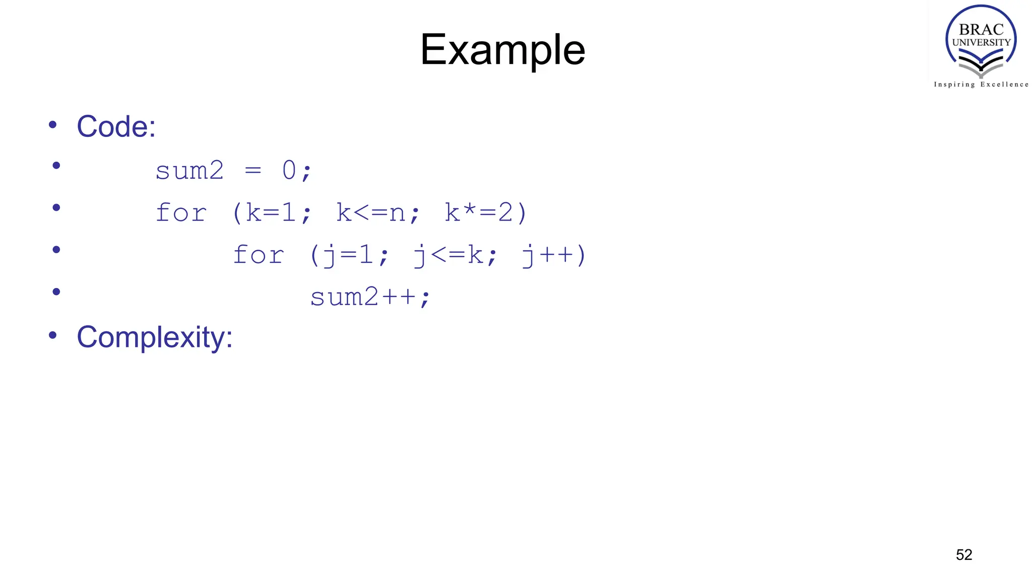
![48
Example
• Code:
• sum = 0;
• for (j=1; j<=n; j++)
• for (i=1; i<=j; i++)
• sum++;
• for (k=0; k<n; k++)
• A[k] = k;
• Complexity:](https://image.slidesharecdn.com/1-250808082021-e09f78bd/75/cse-couse-aefrfrqewrbqwrgbqgvq2w3vqbvq23rbgw3rnw345-48-2048.jpg)

![54
Binary Search
• Given a sorted vector/list a[ ], find the location of element X
unsigned int binary_search(vector<int> a, int X)
{
unsigned int low = 0, high = a.size()-1;
while (low <= high) {
int mid = (low + high) / 2;
if (a[mid] < X)
low = mid + 1;
else if( a[mid] > X )
high = mid - 1;
else
return mid;
}
return NOT_FOUND;
}
• Input size: n = array size()
• Complexity = O( k iterations x (1 comparison+1 assignment) per loop)
= O(log(n))](https://image.slidesharecdn.com/1-250808082021-e09f78bd/75/cse-couse-aefrfrqewrbqwrgbqgvq2w3vqbvq23rbgw3rnw345-54-2048.jpg)