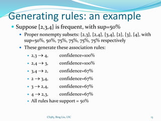
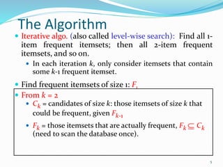
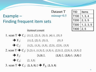
Prof. Neeraj Bhargava
Vishal Dutt
Department of Computer Science, School of
Engineering & System Sciences
MDS University, Ajmer
Many mining algorithms
 There are a large number of them!!
 They use different strategies and data structures.
 Their resulting sets of rules are all the same.
 Given a transaction data set T, and a minimum support and a
minimum confident, the set of association rules existing in T
is uniquely determined.
 Any algorithm should find the same set of rules
although their computational efficiencies and memory
requirements may be different.
 We study only one: the Apriori Algorithm
2
The Apriori algorithm
 The best known algorithm
 Two steps:
 Find all itemsets that have minimum support (frequent
itemsets, also called large itemsets).
 Use frequent itemsets to generate rules.
 E.g., a frequent itemset
{Chicken, Clothes, Milk} [sup = 3/7]
and one rule from the frequent itemset
Clothes  Milk, Chicken [sup = 3/7, conf = 3/3]
3
Step 1: Mining all frequent item sets
 A frequent itemset is an itemset whose support is ≥
minsup.
 Key idea: The apriori property (downward closure
property): any subsets of a frequent itemset are also
frequent itemsets
4
AB AC AD BC BD CD
A B C D
ABC ABD ACD BCD
The Algorithm
 Iterative algo. (also called level-wise search): Find all 1-
item frequent itemsets; then all 2-item frequent
itemsets, and so on.
 In each iteration k, only consider itemsets that contain
some k-1 frequent itemset.
 Find frequent itemsets of size 1: F1
 From k = 2
 Ck = candidates of size k: those itemsets of size k that
could be frequent, given Fk-1
 Fk = those itemsets that are actually frequent, Fk  Ck
(need to scan the database once).
5
Example –
Finding frequent item sets
6
Dataset T TID Items
T100 1, 3, 4
T200 2, 3, 5
T300 1, 2, 3, 5
T400 2, 5
itemset:count
1. scan T  C1: {1}:2, {2}:3, {3}:3, {4}:1, {5}:3
 F1: {1}:2, {2}:3, {3}:3, {5}:3
 C2: {1,2}, {1,3}, {1,5}, {2,3}, {2,5}, {3,5}
2. scan T  C2: {1,2}:1, {1,3}:2, {1,5}:1, {2,3}:2, {2,5}:3, {3,5}:2
 F2: {1,3}:2, {2,3}:2, {2,5}:3, {3,5}:2
 C3: {2, 3,5}
3. scan T  C3: {2, 3, 5}:2  F3: {2, 3, 5}
minsup=0.5
Details: ordering of items
 The items in I are sorted in lexicographic order (which
is a total order).
 The order is used throughout the algorithm in each
itemset.
 {w[1], w[2], …, w[k]} represents a k-itemset w
consisting of items w[1], w[2], …, w[k], where w[1] <
w[2] < … < w[k] according to the total order.
7
Details: the algorithm
Algorithm Apriori(T)
C1  init-pass(T);
F1  {f | f  C1, f.count/n  minsup}; // n: no. of transactions in T
for (k = 2; Fk-1  ; k++) do
Ck  candidate-gen(Fk-1);
for each transaction t  T do
for each candidate c  Ck do
if c is contained in t then
c.count++;
end
end
Fk  {c  Ck | c.count/n  minsup}
end
return F  k Fk; 8
Apriori candidate generation
 The candidate-gen function takes Fk-1 and returns a
superset (called the candidates) of the set of all
frequent k-itemsets. It has two steps
 join step: Generate all possible candidate itemsets
Ck of length k
 prune step: Remove those candidates in Ck that
cannot be frequent.
9
Candidate-gen functionFunction candidate-gen(Fk-1)
Ck  ;
forall f1, f2  Fk-1
with f1 = {i1, … , ik-2, ik-1}
and f2 = {i1, … , ik-2, i’k-1}
and ik-1 < i’k-1 do
c  {i1, …, ik-1, i’k-1}; // join f1 and f2
Ck  Ck  {c};
for each (k-1)-subset s of c do
if (s  Fk-1) then
delete c from Ck; // prune
end
end
return Ck;
CS583, Bing Liu, UIC 10
An example F3 = {{1, 2, 3}, {1, 2, 4}, {1, 3, 4},
{1, 3, 5}, {2, 3, 4}}
 After join
 C4 = {{1, 2, 3, 4}, {1, 3, 4, 5}}
 After pruning:
 C4 = {{1, 2, 3, 4}}
because {1, 4, 5} is not in F3 ({1, 3, 4, 5} is removed)
CS583, Bing Liu, UIC 11
Step 2: Generating rules from frequent
itemsets Frequent itemsets  association rules
 One more step is needed to generate association rules
 For each frequent itemset X,
For each proper nonempty subset A of X,
 Let B = X - A
 A  B is an association rule if
 Confidence(A  B) ≥ minconf,
support(A  B) = support(AB) = support(X)
confidence(A  B) = support(A  B) / support(A)
CS583, Bing Liu, UIC 12
Generating rules: an example
 Suppose {2,3,4} is frequent, with sup=50%
 Proper nonempty subsets: {2,3}, {2,4}, {3,4}, {2}, {3}, {4}, with
sup=50%, 50%, 75%, 75%, 75%, 75% respectively
 These generate these association rules:
 2,3  4, confidence=100%
 2,4  3, confidence=100%
 3,4  2, confidence=67%
 2  3,4, confidence=67%
 3  2,4, confidence=67%
 4  2,3, confidence=67%
 All rules have support = 50%
CS583, Bing Liu, UIC 13
Generating rules: summary
 To recap, in order to obtain A  B, we need to have
support(A  B) and support(A)
 All the required information for confidence
computation has already been recorded in itemset
generation. No need to see the data T any more.
 This step is not as time-consuming as frequent
itemsets generation.
CS583, Bing Liu, UIC 14
On Apriori Algorithm
Seems to be very expensive
 Level-wise search
 K = the size of the largest itemset
 It makes at most K passes over data
 In practice, K is bounded (10).
 The algorithm is very fast. Under some conditions, all
rules can be found in linear time.
 Scale up to large data sets
CS583, Bing Liu, UIC 15

7 algorithm

  • 1.
    Prof. Neeraj Bhargava VishalDutt Department of Computer Science, School of Engineering & System Sciences MDS University, Ajmer
  • 2.
    Many mining algorithms There are a large number of them!!  They use different strategies and data structures.  Their resulting sets of rules are all the same.  Given a transaction data set T, and a minimum support and a minimum confident, the set of association rules existing in T is uniquely determined.  Any algorithm should find the same set of rules although their computational efficiencies and memory requirements may be different.  We study only one: the Apriori Algorithm 2
  • 3.
    The Apriori algorithm The best known algorithm  Two steps:  Find all itemsets that have minimum support (frequent itemsets, also called large itemsets).  Use frequent itemsets to generate rules.  E.g., a frequent itemset {Chicken, Clothes, Milk} [sup = 3/7] and one rule from the frequent itemset Clothes  Milk, Chicken [sup = 3/7, conf = 3/3] 3
  • 4.
    Step 1: Miningall frequent item sets  A frequent itemset is an itemset whose support is ≥ minsup.  Key idea: The apriori property (downward closure property): any subsets of a frequent itemset are also frequent itemsets 4 AB AC AD BC BD CD A B C D ABC ABD ACD BCD
  • 5.
    The Algorithm  Iterativealgo. (also called level-wise search): Find all 1- item frequent itemsets; then all 2-item frequent itemsets, and so on.  In each iteration k, only consider itemsets that contain some k-1 frequent itemset.  Find frequent itemsets of size 1: F1  From k = 2  Ck = candidates of size k: those itemsets of size k that could be frequent, given Fk-1  Fk = those itemsets that are actually frequent, Fk  Ck (need to scan the database once). 5
  • 6.
    Example – Finding frequentitem sets 6 Dataset T TID Items T100 1, 3, 4 T200 2, 3, 5 T300 1, 2, 3, 5 T400 2, 5 itemset:count 1. scan T  C1: {1}:2, {2}:3, {3}:3, {4}:1, {5}:3  F1: {1}:2, {2}:3, {3}:3, {5}:3  C2: {1,2}, {1,3}, {1,5}, {2,3}, {2,5}, {3,5} 2. scan T  C2: {1,2}:1, {1,3}:2, {1,5}:1, {2,3}:2, {2,5}:3, {3,5}:2  F2: {1,3}:2, {2,3}:2, {2,5}:3, {3,5}:2  C3: {2, 3,5} 3. scan T  C3: {2, 3, 5}:2  F3: {2, 3, 5} minsup=0.5
  • 7.
    Details: ordering ofitems  The items in I are sorted in lexicographic order (which is a total order).  The order is used throughout the algorithm in each itemset.  {w[1], w[2], …, w[k]} represents a k-itemset w consisting of items w[1], w[2], …, w[k], where w[1] < w[2] < … < w[k] according to the total order. 7
  • 8.
    Details: the algorithm AlgorithmApriori(T) C1  init-pass(T); F1  {f | f  C1, f.count/n  minsup}; // n: no. of transactions in T for (k = 2; Fk-1  ; k++) do Ck  candidate-gen(Fk-1); for each transaction t  T do for each candidate c  Ck do if c is contained in t then c.count++; end end Fk  {c  Ck | c.count/n  minsup} end return F  k Fk; 8
  • 9.
    Apriori candidate generation The candidate-gen function takes Fk-1 and returns a superset (called the candidates) of the set of all frequent k-itemsets. It has two steps  join step: Generate all possible candidate itemsets Ck of length k  prune step: Remove those candidates in Ck that cannot be frequent. 9
  • 10.
    Candidate-gen functionFunction candidate-gen(Fk-1) Ck ; forall f1, f2  Fk-1 with f1 = {i1, … , ik-2, ik-1} and f2 = {i1, … , ik-2, i’k-1} and ik-1 < i’k-1 do c  {i1, …, ik-1, i’k-1}; // join f1 and f2 Ck  Ck  {c}; for each (k-1)-subset s of c do if (s  Fk-1) then delete c from Ck; // prune end end return Ck; CS583, Bing Liu, UIC 10
  • 11.
    An example F3= {{1, 2, 3}, {1, 2, 4}, {1, 3, 4}, {1, 3, 5}, {2, 3, 4}}  After join  C4 = {{1, 2, 3, 4}, {1, 3, 4, 5}}  After pruning:  C4 = {{1, 2, 3, 4}} because {1, 4, 5} is not in F3 ({1, 3, 4, 5} is removed) CS583, Bing Liu, UIC 11
  • 12.
    Step 2: Generatingrules from frequent itemsets Frequent itemsets  association rules  One more step is needed to generate association rules  For each frequent itemset X, For each proper nonempty subset A of X,  Let B = X - A  A  B is an association rule if  Confidence(A  B) ≥ minconf, support(A  B) = support(AB) = support(X) confidence(A  B) = support(A  B) / support(A) CS583, Bing Liu, UIC 12
  • 13.
    Generating rules: anexample  Suppose {2,3,4} is frequent, with sup=50%  Proper nonempty subsets: {2,3}, {2,4}, {3,4}, {2}, {3}, {4}, with sup=50%, 50%, 75%, 75%, 75%, 75% respectively  These generate these association rules:  2,3  4, confidence=100%  2,4  3, confidence=100%  3,4  2, confidence=67%  2  3,4, confidence=67%  3  2,4, confidence=67%  4  2,3, confidence=67%  All rules have support = 50% CS583, Bing Liu, UIC 13
  • 14.
    Generating rules: summary To recap, in order to obtain A  B, we need to have support(A  B) and support(A)  All the required information for confidence computation has already been recorded in itemset generation. No need to see the data T any more.  This step is not as time-consuming as frequent itemsets generation. CS583, Bing Liu, UIC 14
  • 15.
    On Apriori Algorithm Seemsto be very expensive  Level-wise search  K = the size of the largest itemset  It makes at most K passes over data  In practice, K is bounded (10).  The algorithm is very fast. Under some conditions, all rules can be found in linear time.  Scale up to large data sets CS583, Bing Liu, UIC 15