Assignment 2 GC Article Synthesis – due Sunday February 19.docx
1. Assignment 2: GC Article Synthesis – due Sunday February 19,
2017 by 11:59pm
Read and synthesize a current peer-reviewed research article to
demonstrate your ability to review,
critically analyze, and synthesize scientific information in the
context of global change.
Construct a 300 word (minimum), 2 page paper in which you
outline, summarize AND discuss key concepts
and outcomes of the assigned peer reviewed scientific article in
your own words.
-read the article and actually
highlight the key points (and also
highlight points that you don’t understand so that you can
research those as well) Tip: Think
about the methods, tools, instrumentation, setting of the
research, graphics, and key findings of
the article and synthesize this information.
synthesis (summary of the article).
A great way to begin the writing process is to create several
headings/categories of information
and then use bullet points to outline your thoughts within each
heading. One way to "visualize"
this assignment is to think of how you would recount the main
aspects/details in your own
words to a professor teaching another class who has asked you
2. about current global change
research: e.g. "I was reading an article that focused on...and in
the article the researchers
examined....and mentioned...and their research resulted
in....and..., but also touched on...as
future research".
micropaper (1.5-2pages) that
summarizes the key points of the paper and includes 1) an
introduction 2) several points as your
discussion section and 3) a conclusion paragraph to demonstrate
that you can synthesize and
analyze what you read. You are also expected to research terms
and concepts within the paper
to deepen your understanding AND remember to cite those
sources - as well as the article you
are assigned to synthesize.
must be in the document header
so that it does not interfere with the word count, and the page
number should appear in the
footer of the document (Header/Footer tool is under the
“Insert” menu in Word). 12 font, 1
inch margins. Submissions must be in WORD.DOC format so
that the TAs can easily provide
feedback! Save and submit your file as
“lastname_GC170_Asst2” - e.g. Smith_GC170_Asst2
Assignment 2 Rubric
Assignment 2: GC Article Synthesis – due Sunday February 19,
2017 by 11:59pm
5. .o
rg
/
n
lo
a
d
e
d
fro
m
INTRODUCTION
During the last few decades, it has become evident that because
of a
steadily increasing demand, freshwater scarcity is becoming a
threat to
sustainable development of human society. In its most recent
annual
risk report, the World Economic Forum lists water crises as the
largest
global risk in terms of potential impact (1). The increasing
world pop-
ulation, improving living standards, changing consumption
patterns,
and expansion of irrigated agriculture are the main driving
forces for the
rising global demand for water (2, 3). At the global level and on
an
annual basis, enough freshwater is available to meet such
demand, but
6. spatial and temporal variations of water demand and availability
are large,
leading to water scarcity in several parts of the world during
specific times
of the year. The essence of global water scarcity is the
geographic and
temporal mismatch between freshwater demand and availability
(4, 5),
which can be measured in physical terms or in terms of social or
economic
implications based on adaptation capability (6, 7). Various
studies
have assessed global water scarcity in physical terms at a high
spatial
resolution on a yearly time scale (2, 8–11). Annual assessments
of water
scarcity, however, hide the variability within the year and
underestimate
the extent of water scarcity (12–15). The usually large intra-
annual
variations of both consumption and availability of blue water
(fresh sur-
face water and groundwater) lead to a large variation of water
scarcity
within the year. Wada et al. (13, 14) studied global water
scarcity at a high
spatial resolution on a monthly basis but did not account for
environ-
mental water needs, thus underestimating water scarcity.
Hoekstra et al.
(15) accounted for environmental flow requirements in
estimating global
water scarcity on a monthly basis but did not cover the whole
globe and
used a rather coarse resolution level, namely, the level of river
basins,
7. failing to capture the spatial variation within basins.
Here, we assess global water scarcity on a monthly basis at the
level
of grid cells of 30 × 30 arc min. Water scarcity as locally
experienced is
calculated as the ratio of the blue water footprint in a grid cell
to the
total blue water availability in the cell. Blue water footprint
refers to “blue
water consumption” or “net water withdrawal” and is equal to
the vol-
ume of fresh surface water and groundwater that is withdrawn
and
not returned because the water evaporated or was incorporated
into a
product. Total blue water availability is calculated as the sum of
the runoff
generated within the grid cell plus the runoff generated in all
upstream
grid cells minus the environmental flow requirement and minus
the blue
water footprint in upstream grid cells. We thus account for the
effect of
upstream water consumption on the water availability in
downstream
grid cells. Monthly blue water scarcity (WS) is classified as low
if the blue
water footprint does not exceed blue water availability (WS <
1.0); in this
case, environmental flow requirements are met. Monthly blue
water
scarcity is said to be moderate if it is in the range 1.0 < WS <
1.5, sig-
nificant if it is in the range 1.5 < WS < 2.0, and severe if WS >
2.0.
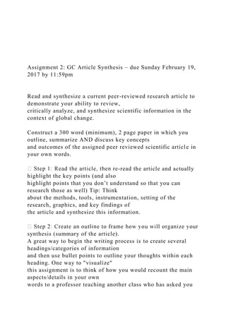
8. Geographic and temporal spread of blue water scarcity
Quarterly averaged monthly blue water scarcities at a spatial
resolution
of 30 × 30 arc min are presented in Fig. 1; annual average
monthly blue
water scarcity is shown in Fig. 2. The 12 monthly water scarcity
maps
are provided in fig. S1 of the Supplementary Materials. Figure 3
shows the
number of months per year in which water scarcity exceeds 1.0.
The
maps in Figs. 2 and 3 show a striking correspondence (with a
correlation
coefficient of 0.99) even if the indicators used are different,
implying that
averaging monthly blue water scarcities over the year suffices
to
capture water scarcity variability within the year.
Year-round low blue water scarcity can be found in the forested
areas
of South America (notably the Amazon basin), Central Africa
(the
Congo basin), and Malaysia-Indonesia (Sumatra, Borneo, New
Guinea)
and in the northern forested and subarctic parts of North
America,
Europe, and Asia. Other places with low water scarcity
throughout the
year can be found in the eastern half of the United States, in
large parts
of Europe, and in parts of South China. Africa shows a band
roughly
between 5° and 15° northern latitude with low water scarcity
from
9. May or June to January but moderate to severe water scarcity
from
February to April. A similar picture is found for the areas
between 10°
and 25° northern latitude, with moderate to severe water
scarcity from
February to May or June in Mexico (Central America) and India
(South
Asia). At higher latitudes, in the western part of the United
States,
Southern Europe, Turkey, Central Asia, and North China, there
are many
areas experiencing moderate to severe water scarcity in the
spring-
summer period. Regions with moderate to severe water scarcity
during
more than half of the year include northern Mexico and parts of
the
western United States, parts of Argentina and northern Chile,
North Africa
and Somalia, Southern Africa, the Middle East, Pakistan, and
Australia.
High water scarcity levels appear to prevail in areas with either
high
population density (for example, Greater London area) or the
presence
of much irrigated agriculture (High Plains in the United States),
or both
(India, eastern China, Nile delta). High water scarcity levels
also occur
in areas without dense populations or intense irrigated
agriculture but
1 of 6
http://advances.sciencemag.org/
10. R E S E A R C H A R T I C L E
o
n
F
e
b
ru
a
ry 9
, 2
0
1
7
h
ttp
://a
d
va
n
ce
s.scie
n
ce
m
a
11. g
.o
rg
/
D
o
w
n
lo
a
d
e
d
fro
m
with very low natural water availability, such as in the world’s
arid areas
(for example, Sahara, Taklamakan, Gobi, and Central Australia
deserts).
Water scarcity in the Arabian Desert is worse than that in other
deserts
because of the higher population density and irrigation
intensity. In
many river basins, for instance, the Ganges basin in India, the
Limpopo
basin in Southern Africa, and the Murray-Darling basin in
Australia,
blue water consumption and blue water availability are
countercyclical,
with water consumption being highest when water availability is
12. lowest.
Large water consumption relative to water availability results in
de-
creased river flows, mostly during the dry period, and declining
lake water
and groundwater levels. Notable examples of rivers that are
fully or nearly
Mekonnen and Hoekstra Sci. Adv. 2016;2:e1500323 12
February 2016
depleted before they reach the end of their course include the
Colorado
River in the western United States and the Yellow River in
North China
(16, 17). The most prominent example of a disappearing lake as
a result
of reduced river inflow is the Aral Sea in Central Asia (18, 19),
but there
are many other smaller lakes suffering from upstream water
consumption,
including, for example, Chad Lake in Africa (19, 20).
Groundwater deple-
tion occurs in many countries, including India, Pakistan, the
United States,
Iran, China, Mexico, and Saudi Arabia (21, 22). Direct victims
of the
overconsumption of water resources are the users themselves,
who in-
creasingly suffer from water shortages during droughts,
resulting in
reduced harvests and loss of income for farmers, threatening the
Fig. 1. Quarterly averaged monthly blue water scarcity at 30 ×
30 arc min resolution. Water scarcity at the grid cell level is
defined as the ratio of the blue
water footprint within the grid cell to the sum of the blue water
generated within the cell and the blue water inflow from
13. upstream cells. Period: 1996–2005.
2 of 6
http://advances.sciencemag.org/
R E S E A R C H A R T I C L E
o
n
F
e
b
ru
a
ry 9
, 2
0
1
7
h
ttp
://a
d
va
n
ce
s.scie
n
14. ce
m
a
g
.o
rg
/
D
o
w
n
lo
a
d
e
d
fro
m
livelihoods of whole communities (2, 23). Businesses depending
on
water in their operations or supply chain also face increasing
risks
of water shortages (1, 24). Other effects include biodiversity
losses,
low flows hampering navigation, land subsidence, and
salinization
of soils and groundwater resources (17, 19, 25, 26).
People facing different levels of water scarcity
15. The number of people facing low, moderate, significant, and
severe water
scarcity during a given number of months per year at the global
level
is shown in Table 1. We find that about 71% of the global
population
(4.3 billion people) lives under conditions of moderate to severe
water
scarcity (WS > 1.0) at least 1 month of the year. About 66%
(4.0 billion
people) lives under severe water scarcity (WS > 2.0) at least 1
month of
the year. Of these 4.0 billion people, 1.0 billion live in India
and another
0.9 billion live in China. Significant populations facing severe
water
scarcity during at least part of the year further live in
Bangladesh
(130 million), the United States (130 million, mostly in western
states
such as California and southern states such as Texas and
Florida), Pakistan
(120 million, of which 85% are in the Indus basin), Nigeria (110
million),
and Mexico (90 million).
The number of people facing severe water scarcity for at least 4
to
6 months per year is 1.8 to 2.9 billion. Half a billion people
face severe
water scarcity all year round. Of those half-billion people, 180
million
live in India, 73 million in Pakistan, 27 million in Egypt, 20
million in
Mexico, 20 million in Saudi Arabia, and 18 million in Yemen.
In the
16. latter two countries, it concerns all people in the country, which
puts those
Mekonnen and Hoekstra Sci. Adv. 2016;2:e1500323 12
February 2016
countries in an extremely vulnerable position. Other countries
in which
a very large fraction of the population experiences severe water
scarcity
year-round are Libya and Somalia (80 to 90% of the population)
and
Pakistan, Morocco, Niger, and Jordan (50 to 55% of the
population).
DISCUSSION
The finding that 4.0 billion people, two-thirds of the world
population,
experience severe water scarcity, during at least part of the
year, implies
that the situation is worse than suggested by previous studies,
which
give estimates between 1.7 and 3.1 billion (see the
Supplementary
Materials) (2, 8, 11–15, 27–30). Previous studies
underestimated water
scarcity and hence the number of people facing severe levels by
assessing
water scarcity (i) at the level of very large spatial units (river
basins),
(ii) on an annual rather than on a monthly basis, and/or (iii)
without
accounting for the flows required to remain in the river to
sustain flow-
dependent ecosystems and livelihoods. Measuring at a basin
scale and
on an annual basis hides the water scarcity that manifests itself
in par-
17. ticular places and specific parts of the year. One or a few
months of
severe water scarcity will not be visible when measuring water
scarcity
annually, because of averaging out with the other, less scarce
months.
We find that the number of people facing severe water scarcity
for at
least 4 to 6 months is 1.8 to 2.9 billion, which is the range
provided
by earlier estimates. Thus, we show that measuring the
variability of water
scarcity within the year helps to reveal what is actually
experienced by
Fig. 2. Annual average monthly blue water scarcity at 30 × 30
arc min resolution. Period: 1996–2005.
Fig. 3. The number of months per year in which blue water
scarcity exceeds 1.0 at 30 × 30 arc min resolution. Period:
1996–2005.
3 of 6
http://advances.sciencemag.org/
R E S E A R C H A R T I C L E
o
n
F
e
b
ru
a
ry 9
19. d
e
d
fro
m
people locally. More than a billion people experience severe
water scar-
city “only” 1 to 3 months per year, a fact that definitely affects
the people
involved but gets lost in annual water scarcity evaluations.
The results are not very sensitive to the assumption on the level
of
environmental flow requirements. With the current assumption
of environ-
mental flow requirements at 80% of natural runoff, we find 4.3
billion
people living in areas with WS > 1.0 at least 1 month in a year.
If we
would assume environmental flow requirements at 60% of
natural run-
off, this number would still be 4.0 billion.
The results are also barely sensitive to uncertainties in blue
water
availability and blue water footprint. We tested the sensitivity
of the
estimated number of people facing severe water scarcity to
changes in
blue water availability and blue water footprint. When we
increase water
availability estimates worldwide and for each month by 20%,
the number
of people facing severe water scarcity during at least 1 month of
20. the year
reduces by 2% (from 4.0 to 3.9 billion). Reducing water
availability by
20% gives 4.1 billion. Changing water footprints in the ±20%
range
results in the number of people facing severe water scarcity to
be be-
tween 3.9 and 4.1 billion as well. Changing water availability in
the
±50% range yields 3.8 to 4.3 billion people facing severe water
scarcity
during at least part of the year, whereas changing water
footprints in
the ±50% range yields 3.6 to 4.2 billion people. The reason for
the low
sensitivity is the huge temporal mismatch between water
demand and
availability: Demand is generally much lower than availability
or the
other way around. Only in times wherein water demand and
availability
Mekonnen and Hoekstra Sci. Adv. 2016;2:e1500323 12
February 2016
are of the same magnitude can changes in one or the other flip
the sit-
uation from one scarcity level to another.
The current study sets the stage for intra-annual water scarcity
mea-
surement. Future improvements in assessing water scarcity can
possibly
be achieved by better accounting for the effect of artificial
reservoirs in
modifying the seasonal runoff patterns and alleviating scarcity.
Besides,
future water scarcity studies should include water consumption
21. related to
the evaporation from artificial reservoirs and interbasin water
transfers,
factors that have not been included in the current study. Future
studies
need to consider scarcity of green water (rainwater that is stored
in the
soil) as well (5, 6, 31–33), assess the interannual variability of
scarcity (13),
develop better procedures to estimate environmental flow
requirements
per catchment (34), and take into account the effect of climate
change,
which most likely will worsen the extent of water scarcity (2).
CONCLUSION
Meeting humanity’s increasing demand for freshwater and
protecting
ecosystems at the same time, thus maintaining blue water
footprints within
maximum sustainable levels per catchment, will be one of the
most
difficult and important challenges of this century (35). Proper
water
scarcity assessment, at the necessary detail, will facilitate
governments,
companies, and investors to develop adequate response
strategies. Water
productivities in crop production will need to be increased by
increasing
Table 1. Number of people facing low, moderate, significant,
and severe water scarcity during a given number of months per
year, for the
average year in the period 1996–2005.
Number of
months per
22. year (n)
Billions of people facing low, moderate, significant, and
severe water scarcity during n months per year
Billions of people
facing moderate or
worse water scarcity
during at least n months
per year
Billions of people
facing severe
water scarcity
during at least n
months per year
Low
water
scarcity
Moderate
water
scarcity
Significant
water
scarcity
Severe water
scarcity
0
0.54
4.98
5.22
2.07
6.04
28. be important that governments and companies formulate water
foot-
print benchmarks based on best available technology and
practice
(38). Assessing the sustainability of the water footprint along
the supply
chain of products and disclosing relevant information will
become in-
creasingly important for investors (39).
o
n
F
e
b
ru
a
ry 9
, 2
0
1
7
h
ttp
://a
d
va
n
ce
s.scie
29. n
ce
m
a
g
.o
rg
/
D
o
w
n
lo
a
d
e
d
fro
m
MATERIALS AND METHODS
Blue water scarcity is calculated per month per grid cell, at a 30
× 30 arc min
resolution, as the ratio of the local blue water footprint (WFloc)
to the
total blue water availability (WAtot) in the month and grid cell
(32)
WS ¼ WFloc
30. WAtot
ð1Þ
Blue water scarcity is time-dependent; it varies within the year
and
from year to year. Blue water footprint and blue water
availability are
expressed in cubic meters per month. For each month of the
year, we
considered the 10-year average for the period 1996–2005. Blue
water
scarcity values were classified into four ranges (15, 32): low
(WS < 1.0),
moderate (1.0 < WS < 1.5), significant (1.5 < WS < 2.0), and
severe
(WS > 2.0). WS = 1.0 means that the available blue water has
been fully
consumed; at WS > 1.0, environmental flow requirements are
not met.
Total monthly blue water availability in a grid cell (WAtot) is
the
sum of locally generated blue water in the grid cell (WAloc)
and the
blue water flowing in from upstream grid cells. Because there
are eco-
nomic activities consuming water in the upstream grid cells, the
blue
water generated upstream is not fully available to the
downstream cell.
Therefore, the blue water available from upstream grid cells is
esti-
mated by subtracting the blue water footprint in the upstream
cells (WFup)
from the blue water generated in the upstream cells (WAup)
31. WAtot ¼ WAloc þ ∑
n
i¼1
ðWAup;i − WFup;iÞ ð2Þ
where the subscript i denotes the cells upstream of the cell
under consid-
eration. If the upstream blue water footprint is larger than the
upstream
available blue water, the total available blue water will be equal
to the lo-
cally available blue water in the grid cell (that is, WAtot =
WAloc). Monthly
blue water availability per grid cell was calculated as the
natural runoff
minus the environmental flow requirement. Natural runoff per
grid cell
was estimated by adding the actual runoff and the blue water
footprint
within the grid cell.
To avoid unrealistic water scarcity values, in particular in the
northern
hemisphere, we have set a condition that when the average
monthly max-
imum temperature is equal to or below 10°C, water scarcity is
set to be
equal to zero. These conditions occur when precipitation and
thus run-
off are very small (sometimes zero or near zero), such that the
WF/WA
ratio can become very large. In practice, this is not experienced
as high
water scarcity, because under these circumstances, water use is
32. generally
small as well (no crop growth in this period) and can be made
available
through small temporary water storage or melting of snow.
Average monthly blue water footprints at a 5 × 5 arc min
resolution
for the period 1996–2005 were derived from Mekonnen and
Hoekstra
(40, 41) and were aggregated to a 30 × 30 arc min resolution.
These data
show the aggregated blue water footprint per grid cell from the
agricultural
(crop and livestock), industrial, and municipal sectors. The blue
water foot-
Mekonnen and Hoekstra Sci. Adv. 2016;2:e1500323 12
February 2016
print of crop production was estimated by considering blue
water con-
sumption per crop per grid cell, based on crop maps, data on
growing
periods, estimated irrigation requirements, and data on actual
irrigation.
The blue water footprints of the industrial and municipal sectors
were
estimated per grid cell based on water consumption data per
country
and population densities.
Monthly actual runoff data at a 30 × 30 arc min resolution were
obtained from the Composite Runoff V1.0 database of Fekete et
al.
(42). Regarding environmental flow requirements, we adopted
the
presumptive environmental flow standard, according to which
80%
33. of the natural runoff is allocated as environmental flow
requirement;
the remaining 20% can be considered as blue water available for
human
use without affecting the integrity of downstream water-
dependent eco-
systems and livelihoods (32, 43). The “flow accumulation”
function of
ArcGIS was used to calculate (rout) blue water availability and
blue
water footprint from upstream to downstream grid cells. The
flow di-
rection raster at a spatial resolution of 30 × 30 arc min was
obtained
from the World Water Development Report II Web site (44, 45).
SUPPLEMENTARY MATERIALS
Supplementary material for this article is available at
http://advances.sciencemag.org/cgi/
content/full/2/2/e1500323/DC1
Supplementary Discussion
Fig. S1. Average monthly blue water scarcity at a spatial
resolution of 30 × 30 arc min.
Table S1. Comparison of results between the current study and
previous studies.
REFERENCES AND NOTES
1. World Economic Forum, Global Risks 2015, 10th Edition
(World Economic Forum, Geneva,
Switzerland, 2015).
2. C. J. Vörösmarty, P. Green, J. Salisbury, R. B. Lammers,
Global water resources: Vulnerability
from climate change and population growth. Science 289, 284–
288 (2000).
3. A. E. Ercin, A. Y. Hoekstra, Water footprint scenarios for
2050: A global analysis. Environ. Int.
34. 64, 71–82 (2014).
4. S. L. Postel, G. C. Daily, P. R. Ehrlich, Human appropriation
of renewable fresh water. Science
271, 785–788 (1996).
5. H. H. G. Savenije, Water scarcity indicators; the deception of
the numbers. Phys. Chem.
Earth B 25, 199–204 (2000).
6. F. R. Rijsberman, Water scarcity: Fact or fiction? Agric.
Water Manage. 80, 5–22 (2006).
7. S. Wolfe, D. B. Brooks, Water scarcity: An alternative view
and its implications for policy and
capacity building. Nat. Resour. Forum 27, 99–107 (2003).
8. T. Oki, Y. Agata, S. Kanae, T. Saruhashi, D. Yang, K.
Musiake, Global assessment of current
water resources using total runoff integrating pathways. Hydrol.
Sci. J. 46, 983–995 (2001).
9. J. Alcamo, T. Henrichs, Critical regions: A model-based
estimation of world water resources
sensitive to global changes. Aquat. Sci. 64, 352–362 (2002).
10. J. Alcamo, P. Döll, T. Hanrichs, F. Kaspar, B. Lehner, T.
Rösch, S. Siebert, Global estimates of
water withdrawals and availability under current and future
“business-as-usual” conditions.
Hydrol. Sci. J. 48, 339–348 (2003).
11. T. Oki, S. Kanae, Global hydrological cycles and world
water resources. Science 313, 1068–1072
(2006).
35. 12. N. Hanasaki, S. Kanae, T. Oki, K. Masuda, K. Motoya, N.
Shirakawa, Y. Shen, K. Tanaka, An
integrated model for the assessment of global water resources—
Part 2: Applications and
assessments. Hydrol. Earth Syst. Sci. 12, 1027–1037 (2008).
13. Y. Wada, L. P. H. van Beek, D. Viviroli, H. H. Dürr, R.
Weingartner, M. F. P. Bierkens, Global
monthly water stress: 2. Water demand and severity of water
stress. Water Resour. Res. 47,
W07518 (2011).
14. Y. Wada, L. P. H. van Beek, M. F. P. Bierkens, Modelling
global water stress of the recent
past: On the relative importance of trends in water demand and
climate variability. Hydrol.
Earth Syst. Sci. 15, 3785–3808 (2011).
15. A. Y. Hoekstra, M. M. Mekonnen, A. K. Chapagain, R. E.
Mathews, B. D. Richter, Global
monthly water scarcity: Blue water footprints versus blue water
availability. PLOS One 7,
e32688 (2012).
5 of 6
http://advances.sciencemag.org/cgi/content/full/2/2/e1500323/D
C1
http://advances.sciencemag.org/cgi/content/full/2/2/e1500323/D
C1
http://advances.sciencemag.org/
R E S E A R C H A R T I C L E
o
n
37. m
16. S. L. Postel, Entering an era of water scarcity: The
challenges ahead. Ecol. Appl. 10, 941–948
(2000).
17. P. M. Vitousek, H. A. Mooney, J. Lubchenco, J. M. Melillo,
Human domination of earth’s
ecosystems. Science 277, 494–499 (1997).
18. W. Shi, M. Wang, W. Guo, Long-term hydrological changes
of the Aral Sea observed by
satellites. J. Geophys. Res. Oceans 119, 3313–3326 (2014).
19. Millennium Ecosystem Assessment, Ecosystems and Human
Well-being: Biodiversity Synthe-
sis (World Resources Institute, Washington, DC, 2005).
20. M. T. Coe, J. A. Foley, Human and natural impacts on the
water resources of the Lake Chad
basin. J. Geophys. Res. 106, 3349–3356 (2001).
21. T. Gleeson, Y. Wada, M. F. P. Bierkens, L. P. H. van Beek,
Water balance of global aquifers
revealed by groundwater footprint. Nature 488, 197–200 (2012).
22. Y. Wada, L. P. H. van Beek, M. F. P. Bierkens,
Nonsustainable groundwater sustaining irri-
gation: A global assessment. Water Resour. Res. 48, W00L06
(2012).
23. UN-Water, FAO, Coping with Water Scarcity: Challenge of
the Twenty-First Century (2007);
www.fao.org/nr/water/docs/escarcity.pdf
38. 24. A. Y. Hoekstra, Water scarcity challenges to business. Nat.
Clim. Change 4, 318–320 (2014).
25. M. Meybeck, Global analysis of river systems: From Earth
system controls to Anthropocene
syndromes. Philos. Trans. R. Soc. London Ser. B 358, 1935–
1955 (2003).
26. FAO, The State of the World’s Land and Water Resources
for Food and Agriculture (SOLAW)—
Managing Systems at Risk (Food and Agriculture Organization
of the United Nations, Rome
and Earthscan, London, 2011).
27. M. Islam, T. Oki, S. Kanae, N. Hanasaki, Y. Agata, K.
Yoshimura, A grid-based assessment of
global water scarcity including virtual water trading. Water
Resour. Manage. 21, 19–33 (2007).
28. M. Kummu, P. J. Ward, H. de Moel, O. Varis, Is physical
water scarcity a new phenomenon?
Global assessment of water shortage over the last two millennia.
Environ. Res. Lett. 5,
034006 (2010).
29. J. Alcamo, T. Henrichs, T. Rösch, World Water in 2025—
Global Modeling and Scenario Anal-
ysis for the World Commission on Water for the 21st Century
(Center for Environmental
Systems Research, University of Kassel, Kassel, Germany,
2000), vol. 2.
30. J. Alcamo, M. Flörke, M. Märker, Future long-term changes
in global water resources driven
by socio-economic and climatic changes. Hydrol. Sci. J. 52,
247–275 (2007).
39. 31. J. Rockström, M. Falkenmark, L. Karlberg, H. Hoff, S. Rost,
D. Gerten, Future water availa-
bility for global food production: The potential of green water
for increasing resilience to
global change. Water Resour. Res. 45, W00A12 (2009).
32. A. Y. Hoekstra, A. K. Chapagain, M. M. Aldaya, M. M.
Mekonnen, The Water Footprint As-
sessment Manual: Setting the Global Standard (Earthscan,
London, 2011).
33. D. Gerten, J. Heinke, H. Hoff, H. Biemans, M. Fader, K.
Waha, Global water availability and
requirements for future food production. J. Hydrometeorol. 12,
885–899 (2011).
34. N. L. Poff, B. D. Richter, A. H. Arthington, S. E. Bunn, R.
J. Naiman, E. Kendy, M. Acreman, C. Apse,
B. P. Bledsoe, M. C. Freeman, J. Henriksen, R. B. Jacobson, J.
G. Kennen, D. M. Merritt,
J. H. O’Keeffe, J. D. Olden, K. Rogers, R. E. Tharme, A.
Warner, The ecological limits of hydrologic
alteration (ELOHA): A new framework for developing regional
environmental flow standards.
Freshwater Biol. 55, 147–170 (2010).
Mekonnen and Hoekstra Sci. Adv. 2016;2:e1500323 12
February 2016
35. A. Y. Hoekstra, T. O. Wiedmann, Humanity’s unsustainable
environmental footprint. Science
344, 1114–1117 (2014).
36. K. A. Brauman, S. Siebert, J. A. Foley, Improvements in
crop water productivity increase water
sustainability and food security—A global analysis. Environ.
Res. Lett. 8, 024030 (2013).
40. 37. J. A. Foley, N. Ramankutty, K. A. Brauman, E. S. Cassidy,
J. S. Gerber, M. Johnston, N. D. Mueller,
C. O’Connell, D. K. Ray, P. C. West, C. Balzer, E. M. Bennett,
S. R. Carpenter, J. Hill, C. Monfreda,
S. Polasky, J. Rockström, J. Sheehan, S. Siebert, D. Tilman, D.
P. M. Zaks,
Solution
s for a
cultivated planet. Nature 478, 337–342 (2011).
38. M. M. Mekonnen, A. Y. Hoekstra, Water footprint
benchmarks for crop production: A first
global assessment. Ecol. Indic. 46, 214–223 (2014).
39. A. Y. Hoekstra, The Water Footprint of Modern Consumer
Society (Routledge, London, 2013).
40. M. M. Mekonnen, A. Y. Hoekstra, National Water Footprint
Accounts: The Green, Blue and
Grey Water Footprint of Production and Consumption (Value of
Water Research Report Se-
ries, no. 50, UNESCO-IHE, Delft, 2011).
41. 41. A. Y. Hoekstra, M. M. Mekonnen, The water footprint of
humanity. Proc. Natl. Acad. Sci. U.S.A.
109, 3232–3237 (2012).
42. B. M. Fekete, C. J. Vörösmarty, W. Grabs, High-resolution
fields of global runoff combining
observed river discharge and simulated water balances. Global
Biogeochem. Cycles 16, 15-1–15-10
(2002).
43. B. D. Richter, M. M. Davis, C. Apse, C. Konrad, A
presumptive standard for environmental
flow protection. River Res. Appl. 28, 1312–1321 (2012).
44. C. J. Vörösmarty, B. M. Fekete, M. Meybeck, R. B.
Lammers, Geomorphometric attributes of
the global system of rivers at 30-minute spatial resolution. J.
Hydrol. 237, 17–39 (2000).
45. C. J. Vörösmarty, B. M. Fekete, M. Meybeck, R. B.
Lammers, Global system of rivers: Its role
in organizing continental land mass and defining land-to-ocean
linkages. Global Biogeochem.
Cycles 14, 599–621 (2000).
42. Acknowledgments: The work was partially developed within the
framework of the Panta Rhei
Research Initiative of the International Association of
Hydrological Sciences. Funding: The work
was fully funded by the University of Twente. Author
contributions: A.Y.H. and M.M.M. designed
the study. M.M.M. performed the modeling work. A.Y.H. and
M.M.M. analyzed the results and
wrote the manuscript. Competing interests: The authors declare
that they have no competing
interests. Data and materials availability: All data needed to
evaluate the conclusions in the pa-
per are present in the paper and/or the Supplementary Materials.
Additional data related to this pa-
per may be requested from the authors. The data used in the
current study are from cited references.
The monthly blue water footprint and scarcity data are available
from the authors upon request.
Submitted 12 March 2015
Accepted 30 November 2015
Published 12 February 2016
10.1126/sciadv.1500323
Citation: M. M. Mekonnen, A. Y. Hoekstra, Four billion people
43. facing severe water scarcity.
Sci. Adv. 2, e1500323 (2016).
e
b
6 of 6
ru
a
ry 9
, 2
0
1
7
http:// www.fao.org/nr/water/docs/escarcity.pdf
http://advances.sciencemag.org/
doi: 10.1126/sciadv.1500323
2016, 2:.Sci Adv
Mesfin M. Mekonnen and Arjen Y. Hoekstra (February 12,
2016)
44. Four billion people facing severe water scarcity
this article is published is noted on the first page.
This article is publisher under a Creative Commons license. The
specific license under which
article, including for commercial purposes, provided you give
proper attribution.
licenses, you may freely distribute, adapt, or reuse theCC BY
For articles published under
. here
Association for the Advancement of Science (AAAS). You may
request permission by clicking
for non-commerical purposes. Commercial use requires prior
permission from the American
licenses, you may distribute, adapt, or reuse the articleCC BY-
NC For articles published under
http://advances.sciencemag.org. (This information is current as
of February 9, 2017):
The following resources related to this article are available
online at
45. http://advances.sciencemag.org/content/2/2/e1500323.full
online version of this article at:
including high-resolution figures, can be found in theUpdated
information and services,
http://advances.sciencemag.org/content/suppl/2016/02/09/2.2.e1
500323.DC1
can be found at: Supporting Online Material
http://advances.sciencemag.org/content/2/2/e1500323#BIBL
7 of which you can access for free at: cites 37 articles,This
article
trademark of AAAS
otherwise. AAAS is the exclusive licensee. The title Science
Advances is a registered
York Avenue NW, Washington, DC 20005. Copyright is held by
the Authors unless stated
published by the American Association for the Advancement of
Science (AAAS), 1200 New
(ISSN 2375-2548) publishes new articles weekly. The journal
isScience Advances