The document summarizes a study analyzing water resources availability and demand in the Mahanadi River Basin in India under projected climate change conditions from 2000 to 2100. The key findings are: 1) A hydrological model is used to project increases in peak runoff during wet months and decreases in average runoff during dry months over the study period, indicating increasing flood risk and drought. 2) Water demand is projected to increase until 2050 due to population growth, then decrease as population growth slows. 3) Some sub-catchments are projected to experience water stress by 2100 based on decreasing availability and demand projections.

1. HYDROLOGICAL PROCESSES
Hydrol. Process. 22, 3589–3603 (2008)
Published online 31 January 2008 in Wiley InterScience
(www.interscience.wiley.com) DOI: 10.1002/hyp.6962
Analysis of water resources in the Mahanadi River Basin,
India under projected climate conditions
Shilpa M. Asokan1
and Dushmanta Dutta2
*
1 Asian Institute of Technology, Thailand
2 School of Applied Science and Engineering, Monash University Gippsland Campus, Churchill, VIC 3842, Australia
Abstract:
The paper presents the outcomes of a study conducted to analyse water resources availability and demand in the Mahanadi
River Basin in India under climate change conditions. Climate change impact analysis was carried out for the years 2000,
2025, 2050, 2075 and 2100, for the months of September and April (representing wet and dry months), at a sub-catchment
level. A physically based distributed hydrologic model (DHM) was used for estimation of the present water availability. For
future scenarios under climate change conditions, precipitation output of Canadian Centre for Climate Modelling and Analysis
General Circulation Model (CGCM2) was used as the input data for the DHM. The model results show that the highest
increase in peak runoff (38%) in the Mahanadi River outlet will occur during September, for the period 2075–2100 and the
maximum decrease in average runoff (32Ð5%) will be in April, for the period 2050–2075. The outcomes indicate that the
Mahanadi River Basin is expected to experience progressively increasing intensities of flood in September and drought in
April over the considered years. The sectors of domestic, irrigation and industry were considered for water demand estimation.
The outcomes of the analysis on present water use indicated a high water abstraction by the irrigation sector. Future water
demand shows an increasing trend until 2050, beyond which the demand will decrease owing to the assumed regulation of
population explosion. From the simulated future water availability and projected water demand, water stress was computed.
Among the six sub-catchments, the sub-catchment six shows the peak water demand. This study hence emphasizes on the
need for re-defining water management policies, by incorporating hydrological response of the basin to the long-term climate
change, which will help in developing appropriate flood and drought mitigation measures at the basin level. Copyright  2008
John Wiley & Sons, Ltd.
KEY WORDS climate change; distributed hydrologic model; general circulation model; water availability and demand; Mahanadi
river basin
Received 4 January 2006; Accepted 25 October 2007
INTRODUCTION
The most widely discussed potential impact of climate
change is on water supply and demand. According to
the Intergovernmental Panel on Climate Change (IPCC,
2001) climate change is defined as any change in cli-
mate over time, due to natural variability or as a result of
anthropogenic activity. Climate change manifests itself
through an elevation in average temperature, variation
in rainfall patterns or an increase in sea level and
thereby affects the water resource availability. Accord-
ing to Alcamo et al. (1997), on a global average, climate
change leads to an increase in annual runoff. About 25%
of the earth’s land area experiences a decrease in runoff,
and this occurs in some countries that are already fac-
ing severe water scarcity. By 2075, the percentage of
world population living in water scarce watersheds is
going to be 69% with climate change, and 74% with-
out climate change conditions. According to the study
by Arnell (1999), average annual runoff will increase in
high latitudes in equatorial Africa and Asia, and south-
east Asia and will show a decrement in mid-latitudes and
* Correspondence to: Dushmanta Dutta, School of Applied Science and
Engineering, Monash University Gippsland Campus, Churchill, VIC
3842, Australia. E-mail: dushmanta.dutta@sci.monash.edu.au
most sub-tropical regions. Runoff regimes in the south
Asian regions are very much influenced by the timing and
duration of the rainy seasons. Rainfall is found exhibiting
an increasing trend over the south Asian region (Mirza
and Ahmed, 2003). Climate change therefore affects river
flows not only through a change in the magnitude of
rainfall but also through possible changes in the onset or
duration of rainy seasons. In developing countries like
India, climate change imposes an additional stress on its
ecological and social systems that are already under pres-
sure due to rapid urbanization, industrialization and eco-
nomic development. India’s greenhouse gas emission is
increasing with its large and growing population. Accord-
ing to Lonergan (1998), India’s climate could become
warmer under conditions of increased atmospheric carbon
dioxide (CO2). The study conducted by Lal et al. (1995)
by taking into account the projected emissions of green-
house gases and sulphate aerosols, predicted an increase
in annual mean, maximum and minimum surface air tem-
peratures by 0Ð7 °C and 1Ð0 °C over land in the 2040s
with respect to the 1980s. India is rich in terms of total
water resources available at the national level. However,
the uneven spatial distribution and temporal dependence
of these resources limits its availability across regions.
The typical seasonality over India as well as the spatial
Copyright  2008 John Wiley & Sons, Ltd.

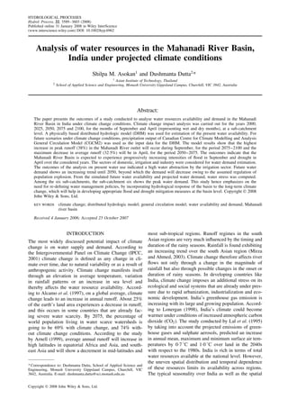
2. 3590 S. M. ASOKAN AND D. DUTTA
variation in the relative dominance of the monsoons is
distinctly reflected in the distribution of most of its cli-
matic elements such temperature, rainfall, etc. as shown
in Figure 1 (Pant and Kumar, 1997).
According to the World Resources Institute (1990),
global withdrawals are expected to rise 2 to 3% annually
until the year 2100. According to Arnell (2000), around
1Ð75 billion people were living in countries suffering
from water scarcity in 2000 (i.e. countries withdrawing
more than 20% of their available water resources each
year). Population growth and economic developments
indicates that by 2025 this could increase to 5 billion peo-
ple (i.e. about 60% of the world’s population). India expe-
rienced a tremendous increase in water demand over the
years because of increasing population complemented by
rapid industrialization. According to the United Nations
Enviroment Programme (UNEP) (Global Environment
Outlook, 2000), if the present consumption patterns con-
tinue, by the year 2025, India may be under high water
stress (more than 40% of total available is withdrawn).
Given the circumstances, the country is presently facing
water stress which is likely to worsen by climate change.
Global, regional and national level studies on water
resources assessment under climate change have been
carried out by several researchers (Frederick et al., 1997;
van Dam, 1999; Lettenmaier et al., 1999; Gleick, 2000;
Figure 1. Mean annual cycles of rainfall and surface air temperature over
India
Vorosmarty et al., 2000; Arora and Boer, 2001; Oki,
2003). Recent approaches on integrated water resources
management emphasize on the significance of river basin
level planning. For long-term planning and management
of water resources under climate change scenarios for
enhancing adaptive capacity to changes, water resources
under climate change should be assessed in basin level
(Arnell, 2004). This study aims to analyse long-term cli-
mate change impact on river flows in the Mahanadi River
Basin, India, which has been reeling through climatic
chaos through out the previous decade. Simultaneously,
water demand is being estimated across the river basin
to identify sub-catchments under water stress. The main
objectives of the study are:
ž to determine present water availability and demand of
Mahanadi basin,
ž to quantify the impact of climate change on water
resources, and
ž to project future water demand and analyse the water
stress in the basin.
MAHANADI RIVER BASIN
The catchment area of the Mahanadi River is
141,589 km2
accounting for 4Ð3% of the total geograph-
ical area of India.
The major part of the Mahanadi River Basin lies in
two provinces: Chhattisgarh (75,136 km2
) and Orissa
(65,580 km2
). Mahanadi River originates from Chhattis-
garh and traverses a length of about 851 km before it
discharges into the Bay of Bengal. Its main tributaries
are the Jira, the Ong, the Ib, and the Tel (Figure 2).
Hirakud Dam, with a gross storage capacity of 7189
MCM, catchment area of 83,400 km2
and command
area of 2639 km2
is the largest dam constructed across
the Mahanadi River. Total amount of renewable water
resources in the basin is 66Ð9 km3
, of which only 30%
is abstracted. The climatic setting is tropical with hot
and humid monsoonal climate. Mahanadi is mainly rain-
fed, and the water availability undergoes large seasonal
fluctuations. Average annual rainfall is 1572 mm, of
Figure 2. Location map of the Mahanadi River Basin
Copyright  2008 John Wiley & Sons, Ltd. Hydrol. Process. 22, 3589–3603 (2008)
DOI: 10.1002/hyp

3. ANALYSIS OF WATER RESOURCES IN THE MAHANADI RIVER BASIN, INDIA 3591
which 70% is precipitated during the south-west mon-
soon between June to October. Rainfall data analysis
indicated the occurrence of peak rainfall during July-
August-September months, which found to abate dur-
ing February-March-April period for the considered time
span from 1990 to 2000. The spatial distribution of rain-
fall pattern of the area highlights the chance of occur-
rence of flood in the downstream sub-catchments, while
upstream sub-catchments sets-off the threat of drought.
This basin is highly vulnerable to flood, and has been
affected by catastrophic flood disasters almost annually.
The monsoon of 2001 topped to the worst hit flood ever
recorded in this basin for the past century, which inun-
dated 38% of its geographical area. Ironically, this basin
suffered one of its worst droughts in the same year, affect-
ing 11 million people, and two-thirds of its area (CSE,
2003).
METHODOLOGY
The study was carried out under the framework presented
in Figure 3. It consisted of five major steps: (i) analysis of
basin-wide surface water availability using a distributed
hydrological model (DHM); (ii) estimation of surface
water availability in future years under climate change
conditions using a DHM driven by general circulation
model (GCM) outputs; (iii) analysis of present water
demand, (iv) estimation of future water demand under
projected socio-economic developments; (v) analysis of
potential impacts of climate changes on water resources
based on the outcomes of previous steps. Year 2000
was considered as the base year of analysis and the
future years selected for analysis were 2025, 2050,
2075 and 2100. According to the Canadian Centre for
Climate Modelling and Analysis General Circulation
Model 2 (CGCM2) A2 scenario, peak rainfall was
projected for the month of September and least value
of average rainfall was projected for the month of April
for the period from 2000 to 2100. Hence the months of
September and April were selected as representative of
the wettest and driest seasons for water availability and
demand computation for the future years.
Distributed Hydrological Model
The Institute of Industrial Science Distributed Hydro-
logical Model (IISDHM) was used for analysis of water
availability at present and for the future situation under
climate change conditions. IISDHM, which was origi-
nally developed at the University of Tokyo, Japan, is
a physically based distributed model consists of five
major flow components of hydrological cycle; inter-
ception and evapotranspiration, unsaturated zone, sat-
urated zone, overland surface flow and river network
flow (Jha et al., 1997; Dutta et al., 2000). The intercep-
tion process is modelled using the concept of Biosphere
Atmosphere Transfer Schemes (BATS) model (Dickin-
son et al., 1993). Evapotranspiration process is solved
using the concept presented by Kristensen and Jensen
(1975). For the unsaturated zone flow, three-dimensional
(3D) Richard’s equation of unsaturated zone is modelled
implicitly (Marsily, 1986). Two-dimensional (2D) Bossi-
nesq’s equation of saturated zone flow is solved implicitly
(Thomas, 1973; Bear and Verruijt, 1987). The original
model used diffusive wave approximation of the 2D
St Venant’s equations of unsteady flow for surface flow
simulation and dynamic wave or diffusive wave approxi-
mation of the one-dimensional (1D) St Venant’s equations
for river network flow. The governing equations of differ-
ent components of the model are presented in Table I. In
this application, the surface and river simulation modules
were simplified using 1D Kinematic-wave approximation
of the St Venant’s equations to reduce computational time
for the large catchment area of the Mahanadi Basin. A
uniform network of square grids is employed to solve the
governing equations with finite difference schemes.
The large amount of spatio-temporal datasets required
for setting up the IISDHM was derived from various
global, regional and local sources. The major spatial
and temporal datasets required for this model are listed
in Table II. The major spatial datasets required include
watershed boundary, topography, landuse, soil, aquifer
layers, river network and cross-sections. The Digital Ele-
vation Model (DEM) for the study area was derived
from the 1 km ð 1 km resolution HYDRO1K dataset
prepared by the United States Geological Survey Depart-
ment (USGS, 2003). The land use dataset was obtained
from a local source (Geoenvitech Private Consultancy,
Orissa), which was derived from LANDSAT TM image
of 1998. Food and Agriculture Organization of the United
Nations (FAO) Soil Database was utilized for extracting
the soil map and characteristics of the basin (FAO Soil
Map, 2003). The river network and cross-section data
Present water availability
estimation using IISDHM
Present water demand
analysis
Future water availability estimation under
climate change effects using IISDHM
driven by precipitation output of GCM
Future water demand
estimation
Analysis of potential impacts of climate change
Figure 3. Research framework
Copyright  2008 John Wiley & Sons, Ltd. Hydrol. Process. 22, 3589–3603 (2008)
DOI: 10.1002/hyp

4. 3592 S. M. ASOKAN AND D. DUTTA
Table I. Governing equations used for different components in IISDHM
Components Governing equations
Interception (BATS concepts),
evapotranspiration (Kristensen and Jensen
equations)
Canopy interception: I D C ð LAI
Actual transpiration: Eat D f1 LAI ð f2 Â ð RDF ð Ep
Actual evaporation:
Es D Ep ð f3 Â C fEp Eat Ep ð f3 Â g ð f4 Â ð f1 f1 LAI g
where, I D intercepted rainfall depth; LAI = leaf area index;
C D parameter dependent on vegetation type; RDF D root distribution
depth; f1 D function of LAI; f2 D function of soil moisture content at
root depth level; and f3 & f4 D functions of soil moisture at top soil
layer.
River flow Mass conservation equation (continuity equation):
(1D St Venant’s equations) ∂Q
∂x C ∂A
∂t D q
and the momentum equation:
∂Q
∂t C ∂
∂x
Q2
A C g ∂z
∂x C Sf D 0
where, t D time; x D distance along the longitudinal axis of watercourse;
A D cross-sectional area; Q D discharge through A; q D lateral
inflow/outflow; g D gravity acceleration constant; z D water surface
level with reference to datum; and Sf D friction slope.
Overland flow (2D St Venant’s equations) Mass conservation equation (continuity equation):
∂uh
∂x C ∂vh
∂y C ∂h
∂t D q
Momentum equations:
In X-direction: ∂u
∂t C u∂u
∂x C v ∂u
∂y C g ∂z
∂x C Sfx D 0
In Y-direction: ∂v
∂t C u∂v
∂x C v ∂v
∂y C g ∂z
∂y C Sfy D 0
where, u D flow velocity in X-direction; v D flow velocity in Y-direction;
z D water head elevation from datum level; Sfx D friction slope in
X-direction; and Sfy D friction slope in Y-direction.
Unsaturated zone (3D Richard’s equation) C
∂
∂t D ∂
∂z [k
∂
∂z C k ] C ∂
∂x [k
∂
∂x ] C ∂
∂y [k
∂
∂y ] Sz
where, D pressure in soil; C D soil water capacity function;
K D unsaturated hydraulic conductivity; and Sz D source or sink
term.
Saturated zone (2D Boussinesq’s equation) ∂
∂x Txx
∂h
∂x C ∂
∂y Tyy
∂h
∂y D S∂h
∂x C Qw Qvert š Qriv Qleakout C Qleakin
where, T D aquifer transmissivity; h D head; t D time; S D aquifer storage
coefficient; Qw D rate of pumping per unit area; Qvert D water entering
from unsaturated zone; Qriv D water inflow from or outflow to river;
Qleakout D rate of leakage going out of layer; and Qleakin D rate of
leakage coming to the layer.
were collected from the Water Resources Department of
the Orissa Province. The main river and the branches
considered in the model are shown in Figure 4. The com-
plex and braiding river network in the delta area was
not included in this analysis as the catchment boundary
derived from HYDRO1K dataset did not include that part
due to its coarse resolution. The river network included
in the model comprises of 15 branches, of which eight
branches have an upstream free end, and one branch has
a downstream free end. DHM was set up with input data
of hourly temporal resolution and spatial resolution of
1 ð 1 km2
. The major temporal datasets required for this
model includes rainfall data, evapotranspiration and soil
parameter data and upstream boundary water level and
discharge data. Rainfall data of daily resolution of six
rain-gauge stations was collected from the Indian Mete-
orological Department, Pune. The spatial distribution of
rainfall pattern of the area highlights the chance of occur-
rence of flood in the downstream sub-catchments, while
upstream sub-catchments sets-off the threat of drought.
Parameters of Kristensen and Jensen equation and Van
Genuchten equation were derived from the evaporation
data, soil and land use categories. The watershed was
divided into six major sub-basins for water resources
analysis. Water level and release at the outlet of Hirakud
Dam was taken as the upstream boundary condition
for calibrating the model for the study area below the
Hirakud Dam, while for calibrating the whole watershed
the recorded water level and discharge data at the gauge
station in the upstream of the catchment was considered
as the upstream boundary condition.
Variables for Water Demand Analysis
The water demand in Mahanadi River Basin was esti-
mated based on three major water utilization sectors;
domestic, industrial and irrigation sectors. These three
sectors were considered in this analysis without tak-
ing into account environmental flow demand. The water
Copyright  2008 John Wiley & Sons, Ltd. Hydrol. Process. 22, 3589–3603 (2008)
DOI: 10.1002/hyp

5. ANALYSIS OF WATER RESOURCES IN THE MAHANADI RIVER BASIN, INDIA 3593
Table II. Input datasets for setting up of IISDHM
Model component Input data requirement
Temporal data Spatial data
Interception and evapotranspiration ž Rainfall ž Landcover
ž Potential evaporation ž Surface roughness
ž Leaf area index
ž Root distribution function
River flow ž U/s and d/s boundary conditions ž River network
ž Water level/discharge ž Branch cross-sections, bed profile
ž River training works
ž Flood control structure
Overland flow ž Rainfall ž Topography
ž Rain gauge locations
ž Detention storage
ž Surface roughness coefficient
Unsaturated zone ž Soil type distribution
ž Hydrogeological properties of soil
ž Initial soil-moisture
Saturated zone ž Groundwater withdrawal ž Aquifer and aquitard layers
ž Hydrogeological properties of aquifer and aquitard
layers
ž Locations of pumping wells
ž Initial groundwater table
Figure 4. Sub-catchment level boundary map of Mahanadi Basin with
river network
demand for each of these sectors was estimated based on
the most relevant socio-economic and demographic char-
acteristics. The most significant variables in determining
domestic water demand are: population (Po) and gross
domestic product (GDP) (G) (Amarsinghe, 2003). The
variables which are significant in determining irrigation
water demand are: irrigated area (A), irrigation efficiency
(Ef), rainfall (R) and evapotranspiration (ETc) (Alcamo
et al., 1997). The significant variables in determining
industrial water demand are: total number of industry (N),
type of industry (T), Industrial GDP (Gi) and number
of employees (E) (Alcamo et al., 1997). These variables
were considered for annual water demands in these three
sectors in the Mahanadi River Basin for present situa-
tion. Secondary data collected from various departments
have been analysed for estimating the water demand of
the considered sectors. For future water demand analysis
in the selected years, projected values of these variables
were considered. The existing projection techniques that
are best suited for the Mahanadi River Basin for differ-
ent variables were used for estimation of the projected
values.
General Circulation Model
The CGCM2 was selected for this study. The CGCM2
is a coupled atmosphere–ocean dynamics model (Flato
et al., 2000). Terrestrial components have 10 vertical
levels discretized by rectangular finite elements. Globally,
the land resolution is about 3Ð75° ð 3Ð75°. Oceans are
modelled on a 1Ð875° ð 1Ð875° grid with 29 vertical
levels. Soils on the land are modelled by using a one-
layer bucket model while accounting for runoff and
soil–water storage with depth that is spatially variable
and depends on soil and vegetation type. Inland lakes, ice
sheets, and soils provide radiation and moisture feedback
from land to the atmosphere. The ocean component
of the model provides sea surface temperatures to the
atmospheric component, and the heat and freshwater flux
is provided to the oceans. Four grids of CGCM2 cover
the entire Mahanadi River Basin as shown in Figure 5.
The selection of GCM was based on several criteria. The
three main criteria were:
ž the performance of the GCM in simulating the present-
day climate in the region;
ž availability of highest resolution data (daily) in public
domain;
ž spatial resolution of the model outputs.
The performance of the selected GCMs [CGCM2, Hadley
Centre Coupled Model, version 3 (HadCM3)] was evalu-
ated by statistical comparison of the model outputs with
Copyright  2008 John Wiley & Sons, Ltd. Hydrol. Process. 22, 3589–3603 (2008)
DOI: 10.1002/hyp

6. 3594 S. M. ASOKAN AND D. DUTTA
Figure 5. CGCM2 grid network and the grids fall over Mahanadi River Basin
observed precipitation data in the target area, and also
over larger scales, to determine the ability of the model
to simulate large scale circulation patterns. A statistical
correlation study was conducted to analyse the represen-
tation of GCM outcomes using long-term ground-based
precipitation data in and around the study area. While
using CGCM2 model, the study area was covered by
four grids but while using the HadCM3 model, the area
fell under two grids. The observed precipitation data
of 4 years from April 1995 to March 1999 was com-
pared with the data taken from the GCM outputs. There
were a total of 20 precipitation gauging stations in the
regional study area. CGCM2 showed highest correlation
with average observed data within the selected grids of
the region for annual and monthly average data compared
to other GCMs. The detailed outcomes of this analy-
sis have been presented in Bhuiyan (2005) and Asokan
(2005).
All of the future climate predictions by GCMs have
uncertainties; one of the uncertainties is due to the
emission scenarios as reported in several studies (Wilby
et al., 1999; Prudhomme et al., 2002; Kay and Reynard,
2006; etc.). Out of the six alternative IPCC scenarios
(IS92a–f), representing a wide array of assumptions
affecting how future greenhouse gas (GHG) emission
might evolve, IS92a forcing scenario has been widely
adopted by the scientific community during the last
decade. In this scenario GHG forcing corresponds to
that observed from 1900 to 1990 and increases at a
rate of 1% per year thereafter, until 2100. The A2
scenario of CCCma CGCM2 was selected in this study
after conducting a preliminary analysis of scenarios
A and B of CCCma CGCM2 and HadCM3. Among
the selected scenarios of CCCma CGCM2, A2 showed
better results (R2
D 0Ð71) and hence was selected for
further projections for the years 2025, 2050, 2075 and
2100.
The study area was covered by four grids of CCCma
CGCM2. Within each GCM grid, a simple downscal-
ing technique was used based on Thiessen polygon
concept. The spatial distribution was carried out using
Thiessen polygons derived from the locations of the
ground based rainfall gauging stations and different
weighing factors different polygons were derived from a
magnitude-distance-elevation model. The raw GCM pre-
cipitation output was multiplied with this factor and that
Copyright  2008 John Wiley & Sons, Ltd. Hydrol. Process. 22, 3589–3603 (2008)
DOI: 10.1002/hyp

7. ANALYSIS OF WATER RESOURCES IN THE MAHANADI RIVER BASIN, INDIA 3595
provided a non-uniform distribution of raw GCM data
for grid of IISDHM and no other bias correction was
applied. This, however, makes the assumption of sta-
tionarity of predictor relations that have been argued
to be problematic (Katz and Parlange, 1996). There
are advanced downscaling techniques such as statisti-
cal downscaling (SD) techniques (Nguyen, 2005; Ghosh
and Mujumdar, 2006). The SD techniques and correc-
tions for elevation biases may further enhance the spa-
tial representation of the GCM outcomes in sub-grid
level.
Calibration and Verification of Hydrological Model
Although the IISDHM is a physically based model,
in absence of the sufficient amount of high resolution
spatial and temporal datasets, the model is required to
be calibrated and verified before an application. In this
analysis, the main calibrated parameter for DHM was
the Manning’s roughness coefficient in the river module.
The model was calibrated against the observed daily dis-
charge at the gauging stations Basantpur (upstream) and
Tikarpara (downstream) for 1998 and verified for 1996.
The range of calibrated values for the Manning’s rough-
ness coefficient was from 0Ð01 to 0Ð05. Figure 6 shows
the comparison between the observed and simulated river
discharge during September 1998 at the Basantpur and
Tikarpara stations at a daily resolution. The simulated
discharge agreed well with the observation at the Basant-
pur station with Nash–Sutcliffe coefficient of 0Ð88. At
the Tikarpara station, the peak value of simulated dis-
charge agreed well with the observation, however the
simulated discharge after the peak was much lower than
the observed values and it did not capture the small peak.
The disagreement may be caused by the return flow from
the irrigated areas, which was not incorporated in the
model. The results of verification of model performance
with the calibrated parameter at the Basantpur and Tilak-
para stations for the period of September 1996 are shown
in Figure 7. The agreements between the observed and
simulated discharge at both the stations were satisfac-
tory with the Nash–Sutcliffe coefficients of 0Ð84 and
0Ð86, respectively. After the satisfactory performance of
the model with the calibrated parameter, it was applied
for flow simulation for 2000 with the observed rain-
fall data and for years 2025, 2050, 2075 and 2100 with
the downscaled rainfall data from the CGCM2. Figure 8
illustrates the trend in simulated precipitation by CGCM2
in the study area. The plot of monthly precipitation shows
an increasing trend in the month of September, and a
decreasing trend in April.
(a)
(b)
Figure 7. Model verification plots for (a) Basantpur and (b) Tikarpara
(a) (b)
Figure 6. Model calibration plots for (a) Basantpur and (b) Tikarpara
Copyright  2008 John Wiley & Sons, Ltd. Hydrol. Process. 22, 3589–3603 (2008)
DOI: 10.1002/hyp

8. 3596 S. M. ASOKAN AND D. DUTTA
(a)
(b)
Figure 8. Rainfall trend of GCM output for (a) September and (b) April
RESULTS AND DISCUSSION
Surface water Availability Estimation
The simulated hourly river discharge at the catch-
ment outlet for the months of September and April
of 2000, 2025, 2050, 2075 and 2100 are shown in
Figures 9 and 10. The simulated results in September
indicated an escalation in river runoff for the future years,
while the results for the month of April showed the
reverse. Figure 11 provides the percentage of increase
and decrease of river discharge for the future years.
The period 2075–2100 shows the maximum percentage
increase in runoff, while a maximum percentage decrease
in runoff is shown during the period 2050–2075. In terms
of sub-catchment level water availability, the maximum
water available is the highest in the sub-catchment six,
which is located close to the delta region, while sub-
catchment one shows the minimum water availability
(Figure 12). The location of sub-catchments, its topog-
raphy, as well as spatial distribution of rainfall supports
this finding.
From an independent analysis carried out by Gosain
and Rao (2003) for estimation of runoff in the Mahanadi
Basin for 40 years using the Regional Climate Model
HadRM2 and a hydrological model; 20 years for the
present situation (1981–2000) and another 20 years for
the future situation (2041–2060), it was found that
Figure 9. Model forecast of water availability of Mahanadi catchment
during September
Figure 10. Model forecast of water availability of Mahanadi catchment
during April
Figure 11. Percentage variation in peak and average discharge
climate change would lead to 28% increase in runoff in
the Mahanadi River Basin. That finding agrees with the
outcome of the present work, which shows an average
26Ð8% increase in runoff for a period of 25 years.
Water availability computed in this study is also
compared with the global water availability study made
by Oki et al. (2001). In this global level study, water
availability was derived from annual runoff estimated
by land surface models using Total Runoff Integrating
Pathways (TRIP), considering the Atmospheric General
Circulation Model (AGCM) of the CCSR/NIES. This
global study followed the difference and ratio method to
obtain the future runoff to downscale the GCM output.
Copyright  2008 John Wiley & Sons, Ltd. Hydrol. Process. 22, 3589–3603 (2008)
DOI: 10.1002/hyp

9. ANALYSIS OF WATER RESOURCES IN THE MAHANADI RIVER BASIN, INDIA 3597
(a) (b)
Figure 12. (a) Sub-catchment level predicted peak runoff for September; (b) sub-catchment level predicted least runoff for April
The comparison found a high deviation of runoff output
between the global and local level studies. Figure 13
illustrates the comparison plot of the global level study
for the year 1995 with the present watershed level study
for the year 2000, and its percentage deviation. The
global level study indicated lower value of river runoff.
All the sub-catchments showed more than 91% lower
values with respect to the watershed level study. To
a certain degree, this high deviation can be attributed
to the different approaches followed, starting from the
DHM to the GCM and most importantly the downscaling
techniques. However, considering the fact that this study
was carried out at watershed level, focusing on local
hydrology, the output can be more representative.
(a)
(b)
Figure 13. (a) Comparison plot of global and watershed level annual
average river runoff; (b) percentage deviation of global level study from
watershed level study
Water Demand Estimation
Population statistics is the crucial player in the esti-
mation procedure of domestic water demand. Sub-
catchmentwise wise demographic data collected from the
Water Resources Department of Orissa Province and cen-
sus data from the Primary Census Abstract of the Office
of the Registrar General of India indicated that 75% of
the total population of Orissa is rural (Orissa Census,
2001). It has been found that surface water demand for
rural population is far ahead than urban. Forty-five per
cent of the rural population is dependant on river water,
as their drinking water source. For urban population it
accounts to only 12%. Groundwater is the other major
water source for urban population.
Estimation of domestic water demand for the future
years necessitates the projection of population of the
study area. The population projection was estimated using
different methods (Isard, 1960) such as the Registrar
General Method of India (RGI), Gibb’s method, curve
fitting method, and was compared with the projected
population values of the Orissa Water Resources Depart-
ment. The curve fitting method showed little similarity
with the existing condition, and hence was excluded
from the study. A comparison plot of RGI, Gibb’s and
Orissa Water Resources department’s projection is shown
in Figure 14. The population projection by the Water
Resources department followed the Exponential Growth
Rate method with an assumption of zero population
Figure 14. Population projection using different techniques
Copyright  2008 John Wiley & Sons, Ltd. Hydrol. Process. 22, 3589–3603 (2008)
DOI: 10.1002/hyp

10. 3598 S. M. ASOKAN AND D. DUTTA
growth rate by 2050 to meet their State Planning. RGI
method showed a huge increase in population because of
the fact that this method considers an increase in popula-
tion per person per year basis. Gibb’s method indicated
low value of population compared to other techniques. By
considering these three projections, the projected popula-
tion by Orissa Water Resources department was found to
be the most acceptable since it was not showing extrem-
ities, and hence the same was selected in this study. By
incorporating the Chhatishgarh segment of population,
the future projection was made up to 2101 (Tables III
and IV). In order to estimate domestic water demand on
a rural and urban basis, the percentage migration from
rural to urban was estimated from the historical datasets.
The migration was 19% during 1971–1981 and 32% in
1981–1991, a 6% increase in migration was noticed for
the Mahanadi watershed as a whole. However, this total
migration cannot be considered as the same for the indi-
vidual sub-catchments because of the fact that the degree
of migration from each of these sub-catchments varied
depending on their development status. Hence, the per-
centage of migration for individual sub-catchments was
considered in the analysis without taking into account
inter-basin migration due to lack of such statistics. This
increase in migration is considered as constant through-
out and the urban population is estimated for the years
2025, 2050, 2075 and 2100 based on 2000 data. From
the projected total population, and projected urban popu-
lation, the projected rural population was computed. Total
domestic water demand was estimated from the rural and
urban water demands, considering their respective per
capita water use. According to the Planning Commission
of the Government of India, for year 1999 water with-
drawal per person in the urban area was 135 litres per
day, and in rural areas it was 40 litres per day. How-
ever, the World Health Organization (WHO) standards
emphasize on a minimum of 70 litres per day per capita
taking into account proper sanitation. The Millennium
Development Goals of the United Nations also aims in
providing about 1Ð5 million people with access to safe
water and 2 billion with access to basic sanitation facil-
ities between 2000 and 2015. Therefore, a scenario was
considered in this study assuming rural water demand
to increase so as to meet the WHO (2004) standards
in the year 2025, and further improve the per capita
water availability status. The International Food Policy
Research Institute (IFPRI) projects domestic water use in
India to double between 1995 and 2025 (IFPRI, 2002).
This factor was considered in improving urban per capita
water demand in the future years. Figure 15 illustrates
the projected domestic water demand.
Industrial water demand data was collected from the
Water Resources department of Orissa and analysed
on a sub-catchment basis for the year 2001. For sub-
catchments two, three and five analysis was carried
out separately, however, the analysis was carried out
together for sub-catchments one, four and six due to lack
Figure 15. Projected domestic water demand
Table III. Projected demography from 1991 to 2041
Sub-catchment 1991 2001 2011 2021 2031 2041
1 9,528,406 11,153,226 13,055,159 15,281,431 17,887,348 20,937,647
2 1,572,723 1,840,910 2,154,836 2,522,296 2,952,419 3,455,890
3 1,288,934 1,508,728 1,766,008 2,067,162 2,419,671 2,832,294
4 2,465,295 2,885,686 3,377,776 3,953,782 4,628,013 5,417,221
5 3,349,237 3,920,362 4,588,891 5,371,427 6,287,407 7,359,588
6 1,314,519 1,538,676 1,801,062 2,108,194 2,467,701 2,888,514
Total 19,519,114 22,847,588 26,743,732 31,304,292 36,642,559 42,891,154
Table IV. Projected demography from 2051 to 2101
Sub-catchment 2051 2061 2071 2081 2091 2101
1 24,508,109 24,508,109 24,508,109 24,508,109 24,508,109 24,508,109
2 4,045,217 4,045,217 4,045,217 4,045,217 4,045,217 4,045,217
3 3,315,280 3,315,280 3,315,280 3,315,280 3,315,280 3,315,280
4 6,341,010 6,341,010 6,341,010 6,341,010 6,341,010 6,341,010
5 8,614,606 8,614,606 8,614,606 8,614,606 8,614,606 8,614,606
6 3,381,088 3,381,088 3,381,088 3,381,088 3,381,088 3,381,088
Total 50,205,310 50,205,310 50,205,310 50,205,310 50,205,310 50,205,310
Copyright  2008 John Wiley & Sons, Ltd. Hydrol. Process. 22, 3589–3603 (2008)
DOI: 10.1002/hyp

11. ANALYSIS OF WATER RESOURCES IN THE MAHANADI RIVER BASIN, INDIA 3599
Figure 16. Industrial water demand for sub-basins (a) six, four and one, (b) three, (c) five and (d) two for 2001
of data at sub-catchment level. In 2001, the maximum
industrial water demand was for sub-catchment three,
and the minimum was for sub-catchment two. The sector
demanding major share of water is the thermal power
industry, which is followed by the aluminium industry
(Figure 16).
From the observed industry water demand rate from
1981 to 2001, and by keeping the growth rate as con-
stant, future demand rates were predicted. From the pro-
jected demand rate, future industrial water demand was
estimated (Table V). At this point it could be argued
that the future industrial water demand may differ sig-
nificantly from today’s because of improved technolo-
gies and increase water-use efficiency. Nevertheless, an
increased use of recycled water could further reduce total
industrial withdrawals. Gleick (1997) and Shiklomanov
(1993, 1998) also support this view of decrease in overall
consumptive use due to improvements in industrial re-use
of water.
The present irrigation water demand of the basin
was estimated by considering the present and future
irrigation projects of the basin. Figure 17 illustrates the
Table V. Projected industry water demand (ð106
m3
)
Sub-catchment 2001 2025 2050 2075 2100
1 0Ð803 0Ð803 0Ð803 0Ð803 0Ð803
2 3Ð99 4Ð49 4Ð99 5Ð49 5Ð99
3 3Ð19 3Ð73 4Ð64 6Ð264 9Ð396
4 1Ð043 1Ð05 1Ð059 1Ð067 1Ð07
5 216Ð57 217Ð65 220Ð16 222Ð66 225Ð17
6 2Ð13 2Ð134 2Ð141 2Ð149 2Ð159
Figure 17. Irrigation water demand for 2001
sub-catchment level irrigation water demand for the year
2001. Figure 17 shows that sub-catchment four holds
the major stake of irrigation water. The irrigation water
demands for the selected future years were estimated
by incorporating the estimated water demands for the
irrigation projects which are proposed to be completed in
the coming years. The change in irrigation intensity was
also considered depending on the possible changes in land
use during the future years. For the sub-catchments six
and four, the percentage of increase in irrigation water
demand from 2001 to 2051 is 5Ð31 to 23% (according
to water balance scenario of Hirakud Dam for the year
2051, projected by Water Resources Department, Orissa),
which accounts to a 3Ð3% increase. Therefore, for the
periods 2001–2025 and 2025–2050, the percentage of
increase in irrigation is taken as 1Ð65%. Also, a similar
rate of increase is assumed for 2075 and 2100. For
Copyright  2008 John Wiley & Sons, Ltd. Hydrol. Process. 22, 3589–3603 (2008)
DOI: 10.1002/hyp

12. 3600 S. M. ASOKAN AND D. DUTTA
sub-catchment three, where irrigation area is less, and
major occupation is mining, the chance of irrigation
intensification in the coming years will be less. Hence
a 0Ð5% increase of irrigation rate is assumed. Sub-
catchments five and two are large open and degraded
forest area. Here the trend of deforestation is high and
this amplifies the chance of increase in irrigated area in
the future years. Therefore a 1Ð2% increase in irrigation
demand is assumed for future years, considering that the
probability of irrigation intensification here will be less
than sub-catchments six and four. Presently there are no
irrigation projects in sub-catchment one, and the chance
of having any in the future years is also less because
of its hilly topography. Considering all these factors into
account irrigation water demands for the future years are
projected (Figure 18).
From the earlier analysis, it has been found that the
major share of the total water demand is contributed
by the irrigation sector. About 90% of the total water
abstraction is for the irrigation sector. According to
Clarke (2003), the heaviest water user globally is agri-
culture, accounting for about 69% of total global water
abstraction. A higher percentage of demand in irrigation
water in this part of the world can be owed to the agri-
culture oriented backbone of developing India. Hence,
even a low degree of change in the irrigation management
practice followed in the region can lead to a detectable
variation in water demand domain for the future years.
Sub-catchment six is the major stakeholder accounting to
74Ð7% of the total demand. Sub-catchment four stakes
22% of the total. The demand side of the remaining sub-
catchments is negligible.
Total water abstraction computed in the present study
is compared with water abstraction values indicated by
the global level assessment of water resources study made
by Oki et al. (2001). The comparison is made on a sub-
catchment level for the years 1995 and 2050 (Figure 19).
The global study showed a very high deviation from the
local watershed based analysis. For sub-catchments one,
two, three, four, five and six the percentage negative
deviation was 68, 65, 85, 80, 85 and 92%, respectively.
Comparison for the year 2050 is showing less deviation
when compared to present, for sub-catchments one, two,
three and five. For the remaining sub-catchments, the
Figure 18. Projected irrigation water demand
Figure 19. (a) Comparison plot of global and watershed based study for
1995; (b) percentage deviation of 1995 and 2050 total water abstraction
obtained from global study with respect to present watershed level study
deviation is more when compared to 1995. To be concise,
the global level water abstraction output pacifies the
original critical situation, which can be more accurately
interpreted through a watershed level analysis.
Climate Impact Analysis
Complementary to the information on the contempo-
rary water balance of the basin, an in-depth interpretation
of future water balance was carried out, explicating the
condition arising in the future due to an excessive or
limited surface water supply. Thereby the effect of an
increasing future water demand on the unsteady water
availability of the Mahanadi River Basin under climate
change conditions is interpreted.
The month of September is expected to experience
an excess of water which is found to be escalating in
the future years. Figure 20 shows the increasing trend
of excess runoff (runoff after meeting water demand)
of the Mahanadi Basin at the catchment outlet during
September. In order to analyse how the increasing water
pour at the mouth of Mahanadi is going to affect the
population, it is necessary to know the flood history
of Mahanadi. Floods in the Mahanadi River start when
water discharge mounts to 17,150 m3
s 1
. A discharge of
28,580 m3
s 1
may result in damaging floods (Mohanti,
2003). The years 2001 and 2003 marked very high floods
Copyright  2008 John Wiley & Sons, Ltd. Hydrol. Process. 22, 3589–3603 (2008)
DOI: 10.1002/hyp

13. ANALYSIS OF WATER RESOURCES IN THE MAHANADI RIVER BASIN, INDIA 3601
Figure 20. Plot of excess discharge of the Mahanadi Basin
in the Mahanadi River. The highest discharge recorded
was 40,868 m3
s 1
. The extent of damage brought about
by 2001 flood is tabulated in Table VI (UNDMT, 2001).
It explains the degree of catastrophe experienced by
the population because of a destructive flood which
lasted only for a couple of days. The findings of the
current study are pointing towards the future possibility
of floods during the month of September with an even
higher magnitude because of climatic change. Therefore,
apposite flood management measures have to be taken
well in advance to save the population, especially those
thriving in the delta region. Looking at the contemporary
and successive water stress factor for the Mahanadi
Basin, it is found that sub-catchment one shows the
largest amount of shortage of 467 MCM for 2000.
All other sub-catchments show water shortage volume
ranging from 56 to 160 MCM (Figure 21). Figure 22
shows the percentage increase in water demand and
the percentage decrease in water availability for the
future years. It can be observed from Figure 22 that the
percentage decrease in water availability is maximum
during the period 2050–2075. However, the percentage
increase in water demand shows a negative trend during
the same period. This in effect pacifies the intensity of
water stress in the basin during the same period. All the
sub-catchments are growing towards a high degree of
scarcity during the period from 2000 to 2050. However,
beyond 2050 the intensity of scarcity is seen alleviated.
The main reason behind this is the reduction in water
demand beyond 2050 owing to the zero growth rate
in population assumed to be attained according to the
planning propaganda of the state. Figure 23 shows the
water stress projected for the year 2100 and the per capita
water availability under this projected stress conditions.
From the per capita water availability illustrated in
Figure 23, it is clear that all the sub-catchments are under
water stress. Within this stress realm, sub-catchments
one and three can be considered as under peak stress,
because the per capita water availability for these sub-
catchments is even less than 5% of the maximum per
capita water availability with respect to the whole basin.
Sub-catchments four, five and two can be considered
as under medium stress since the per capita water
availability in these sub-catchments is varying from 10
to 30% of the maximum value. Sub-catchment six, which
is having the maximum per capita water availability of
4Ð41 litres per day, can be considered as under low stress.
In recent years, the Mahanadi River Basin is experi-
encing drought in the same region, which was flooded
at some point of time. It has already been mentioned
that this river basin experienced the peak flood in the
year 2001. The basin also experienced the worst hit
drought also in the same year. Western Orissa districts
were mainly affected. Media reported about 16 starvation
deaths. Migration of people from the drought stricken
areas to the neighbouring states of Madhya Pradesh,
Maharashtra, and Gujarat was also observed during this
period (UN, 2001). The present study predicts an increas-
ing trend of water scarcity in the dry season all through
Table VI. Flood damage tabulated for 2001 flood
Sl no. Particular Loss
1 Death toll 39
2 Flood affected population 5Ð978 million
3 Number of districts affected 24
4 Number of blocks affected 149
5 Number of panchayats affected 1596
6 Number of villages affected 9151
7 Number of houses damaged 27,632
8 Crop loss 0Ð00375 million km2
9 Crop loss estimated US$5 million
Figure 21. Water shortage for the year 2000
Figure 22. Percentage variation in water availability and demand
Copyright  2008 John Wiley & Sons, Ltd. Hydrol. Process. 22, 3589–3603 (2008)
DOI: 10.1002/hyp

14. 3602 S. M. ASOKAN AND D. DUTTA
Figure 23. Sub-catchment level projected water shortage for 2100
the coming decades. This necessitates appropriate water
harvesting techniques during the peak season to save
water, which would have otherwise be lost in the sea.
CONCLUSIONS
Climate change has the potential to alter the adequacy and
frequency of precipitation leading to a sporadic hydro-
logic cycle, the climax of which can be reflected in the
water supply and demand aspects. The present study pro-
vides an assessment of the impact of climate change on
water resources of the Mahanadi River Basin throughout
the twenty-first century. A DHM driven by GCM output
was used in this study to forecast present and future water
availability. The future water availability forecast indi-
cated an escalating trend in river runoff thereby alarm-
ing flood in this highly climatically vulnerable basin for
the month of September. The outcomes of the analysis
for the month of April however indicate an accelerating
water scarcity in the future. The finding of the analy-
sis on present scenario water demand indicates a high
water abstraction by the irrigation sector. Among the
six sub-catchments, sub-catchment six shows the peak
water demand. The future water demand is projected
from the contemporary state using appropriate projection
techniques, and it is observed that the demand is increas-
ing until 2050, beyond which the demand will decrease
owing to the assumed regulation of population. Region
of Mahanadi under peak stress is predicted and per capita
water availability under stress condition is estimated. This
study hence reveals the vulnerability of the Mahanadi
River Basin to climate change. The output from this study
can be considered as a guideline for the policy-makers to
plan and prepare for future floods and droughts.
The study has presented a framework of comprehen-
sive analysis of impacts of climate change in water
resources at river basin scale such that outcomes of the
study can be directly utilized for decision-making pro-
cess. The large scale heterogeneity in water resources
in countries like India underlies the importance of sub-
basin scale comprehensive understanding of impacts of
climate change. The generic methodology used in the
study can be transferred to any other river basins for
analysing impacts of climate change in water resources
towards adaptive management.
The accuracy of future water availability forecast
depends on the GCM projections used. The major prob-
lem in applying GCM projections to finer area assessment
is that the coarse resolution of the data may not realisti-
cally represent the orography and land surface processes
leading to deviation of observed and modelled rain-
fall pattern. Hence appropriate downscaling techniques
need to be followed. This study looked into the quan-
tity aspects of surface water resources under climatic
variation. The conjunctive use of surface and groundwa-
ter resources with adequate allowance for environmental
should be included for enhancement of the findings for
water resources management.
REFERENCES
Amarasinghe U. 2003. Spatial variation in water supply and demand
across the River Basins of India, Draft Research Report, IWMI,
Colombo, Sri Lanka. Available at http://www.icid.org/report upali
nov03.pdf.
Arnell NW. 1999. Climate change and global water resources. Global
Environmental Change S31–S49.
Arnell NW. 2000. Global climate change and water resources: to 2025
and beyond. In An ODI (The Overseas Development Institute)-SOAS
(The School of Oriental and African Studies) Meeting Series Leading
Copyright  2008 John Wiley & Sons, Ltd. Hydrol. Process. 22, 3589–3603 (2008)
DOI: 10.1002/hyp

15. ANALYSIS OF WATER RESOURCES IN THE MAHANADI RIVER BASIN, INDIA 3603
up to the Second World Water Forum and Ministerial Conference,
Overseas Development Institute, February 2000; 17–22.
Arnell NW. 2004. Climate change and global water resources: SRES
emissions and socio-economic scenarios. Global Environmental
Change 14: 31–52.
Alcamo J, Doll P, Kaspar F, Siebert S. 1997. Global Change and Global
Scenarios of Water Use and Availability: An Application of Water GAP
1Ð0. Center for Environmental Systems Research (CESR), University
of Kassel: Kassel.
Arora VK, Boer GJ. 2001. Effects of simulated climate change on the
hydrology of major river basins. Journal of Geophysical Research
106(D4): 3335–3348.
Asokan SM. 2005. Water resources analysis under projected climate
conditions in the Mahanadi River Basin, India. MEng thesis, No.WM-
04-13, Asian Institute of Technology, Thailand; 87 pp.
Bear J, Verruijt A (ed.). 1987. Modeling Ground Water Flow and
Pollution. D. Reidel Publishing Company: Dordrecht.
Bhuiyan JAB. 2005. Assessment of the economic impacts of floods under
climate change conditions in a coastal city in Bangladesh. MEng thesis,
No. WM-04-12, Asian Institute of Technology, Thailand; 113 pp.
CSE. 2003. Climate Change and Orissa, Factsheet, Global Environmental
Negotiations. Available at http://www.cseindia.org/programme/geg/
pdf/orissa.pdf (accessed September 15, 2005).
Clarke R. 2003. Water Crisis? OECD Observer. Available at
http://www.oecdobserver.org/news/fullstory.php/aid/935/Water
crisis .html (accessed September 10, 2005).
Dickinson R, Sellers AH, Kennedy PJ. 1993. Biosphere Atmosphere
Transfer Schemes (BATS) as coupled to the Community Climate Model,
NCAR Technical Note, NCAR/TN-383CSTR, National Center for
Atmospheric Research: Boulder, CO.
Dutta D, Herath S, Musiake K. 2000. Flood inundation simulation in
a river basin using a physically based distributed hydrologic model.
Hydrological Processes 14: 497–519.
Food and Agriculture Organization of the United Nations (FAO)
Soil MAP. 2003. Available at http://www.fao.org/ag/agl/agll/wrb/
mapindex.stm (accessed October 28, 2005).
Flato GM, Boer GJ, Lee WG, McFarlane NA, Ramsden D, Reader MC,
Weaver AJ. 2000. The Canadian centre for climate modeling and
analysis global coupled model and its climate. Climate Dynamics 16:
451–467.
Frederick KD, Major DC, Stakhiv EZ. (eds). 1997. Climate Change and
Water Resources Planning Criteria. Kluwer Academic: Norwell, MA.
Ghosh S, Mujumdar PP. 2006. Future rainfall scenario over Orissa with
GCM projections by statistical downscaling, Current Science 90(3):
396–404.
Gleick PH. 1997. Water 2050: Moving Toward a Sustainable Vision
for the Earth’s Fresh Water. Working Paper of the Pacific Institute
for Studies in Development, Environment, and Security, Oakland,
California. Prepared for the Comprehensive Freshwater Assessment for
the United Nations General Assembly and the Stockholm Environment
Institute, Stockholm, Sweden.
Gleick PH. 2000. Water: The Potential Consequences of Climate
Variability and Change for the Water Resources of the United States. US
Global Change Program. Pacific Institute for Studies in Development,
Environment, and Security: Oakland, CA.
Global Environment Outlook. 2000. Fresh water. UNEP, The
state of the environment, Regional Synthesis. Available at
http://www.unep.org/geo2000/english/0046.htm (accessed October 12,
2005).
Gosain AK, Rao S. 2003. Impacts of climate change on water sector. In
Climate Change and India: Vulnerability Assessment and Adaptation,
Shukla PR, Sharma SK, Ravindranath NH, Garg A, Bhattachatya S
(eds). Universities Press: Andhra Pradesh.
International Food Policy Research Institute (IFPRI). 2002. Global
Water Outlook to 2025: Averting an Impending Crisis. Available
at http://www.ifpri.org/media/water countries.htm#india [January 15
2005].
Intergovernmental Panel on Climate Change (IPCC). 2001. Climate
Change 2001: Impacts, Adaptation and Vulnerability. Contribution of
Working Group II to the Third Assessment Report of the IPCC.
Cambridge University Press: Cambridge.
Isard W. 1960. Methods of Regional Analysis. In Population Projection,
The MIT Press: Cambridge, MA; 5–33.
Jha R, Herath S, Musiake K. 1997. Development of IIS Distributed
Hydrological Model (IISDHM) and its application in Chao Phraya
River Basin, Thailand. Annual Journal of Hydraulic Engineering,
JSCE, 41: 227–232.
Katz RW, Parlange MB. 1996. Mixtures of stochastic processes:
application to statistical downscaling. Climate Research 7: 185–193.
Kay AL, Reynard NS. 2006. RCM rainfall for UK flood frequency
estimation. I. Method and validation. Journal of Hydrology 318(1–4):
151–162.
Kristensen K, Jensen S. 1975. A model for estimating actual evapo-
transpiration from potential evapotranspiration. Nordic Hydrology 6:
70–88.
Lal M, Cubasch U, Voss R, Waszkewitz J. 1995. Effect of transient
increase in greenhouse gases and sulphate aerosols on monsoon.
Current Science 69(9): 752–763.
Lettenmaier DP, Wood AW, Palmer RN, Wood EF, Stakhiv EZ. 1999.
Water resources implications of global warming: A U.S. regional
perspective. Climate Change 43: 537–579.
Lonergan S. 1998. Climate warming and India. In Measuring the Impact
of Climate Change on Agriculture, Dinar A (ed.), World Bank Technical
Paper No. 402. The World Bank: Washington, DC.
Marsily CD. 1986. Quantitative Hydrogeology, Academic Press: New
York.
Mirza MMQ, Ahmed AU. 2003. Climate changes and water resources
in South Asia: Vulnerabilities and coping mechanisms—a synthesis.
In Climate Change and Water Resources in South Asia, Muhammed A
(ed.). Asian-Pacific Network (APN): Kobe.
Mohanti M. 2003. Mahanadi river delta, east coast of India:
an overview on evolution and dynamic processes. Available at
http://www.megadelta.ecnu.edu.cn/main/upload/mahanadi.pdf
(accessed September 12, 2005).
Nguyen VTV. 2005. Downscaling methods for evaluating the impacts of
climate change and variability on hydrological regime at basin scale. In
Proceedings of the International Symposium on Role of Water Sciences
in Transboundary River Basin Management, Thailand; 1–8.
Orissa Census. 2001. Primary Census Abstract, Census of India. Office
of the Registrar General: New Dehli.
Oki T. 2003. Global water resources assessment under climatic change
in 2050 using TRIP. Water resources systems—water availability
and global change. In Proceedings of Symposium HS02a held during
IUGG2003 at Sapporo, IAHS Publication No. 280. IAHS Press:
Wallingford.
Oki T, Agata Y, Kanae S, Saruhashi T, Yang D, Musiake K. 2001.
Global assessment of current water resources using Total Runoff
Integrating Pathways. Hydrological Sciences 46(6): 983–995.
Pant GB, Kumar KR. 1997. Climates of South Asia. John Wiley and Sons:
Singapore; 18.
Prudhomme C, Reynard M, and Crooks S. 2002. Downscaling of global
climate models for flood frequency analysis: where are we now?
Hydrological Processes 16: 1137–1150.
Shiklomanov IA. 1993. World fresh water resources. In Water in Crisis: A
Guide to the World’s Fresh Water Resources. Gleick PH (ed.). Oxford
University Press: New York.
Shiklomanov IA. 1998. Assessment of water resources and water
availability in the world. Report for the Comprehensive Assessment of
the Freshwater Resources of the World, United Nations. Data archive
on CD-ROM from the State Hydrological Institute, St Petersburg,
Russia.
Thomas R. (ed.). 1973. Ground Water Models. FAO: Rome.
UNDMT Situation Report. 2001. Orissa Floods 2001. Avail-
able at http://www.un.org.in/dmt/orissa/072001flood/sitreps/ (accessed
September 5, 2005).
United Nations (UN). 2001. Situation report on Orissa drought 2001.
Available at http://www.un.org.in/dmt/orissa/ (accessed August 30,
2005).
US Geological Survey (USGS). 2003. Land processes distributed active
archive centre. Available at http://edcdaac.usgs.gov/gtopo30/hydro/
asia.asp (accessed September 30, 2005).
van Dam JC. (ed.) 1999. Impacts of Climate Change and Climate
Variability on Hydrologic Regimes. Cambridge University Press: New
York.
Vorosmarty CJ, Green P, Salisbury J, Lammers RB. 2000. Global water
resources: vulnerability from climate change and population growth.
Science 289: 284–288.
Wilby RL, Hay LE, Leavesley GH. 1999. A comparison of downscaled
and raw GCM output: implications for climate change scenarios in the
San Juan River Basin, Colorado. Journal of Hydrology 225: 178–191.
World Health Organization (WHO). 2004. Minimum Water Quantity
Needed for Domestic Uses. WHO Regional Office for South-east Asia:
New Dehli.
World Resources Institute. 1990. World Resources 1990–91. Oxford
University Press: New York.
Copyright  2008 John Wiley & Sons, Ltd. Hydrol. Process. 22, 3589–3603 (2008)
DOI: 10.1002/hyp