


The document describes data envelopment analysis (DEA), a quantitative technique for measuring the efficiency of decision making units (DMUs) that may have multiple inputs and outputs. DEA formulates a linear programming problem to determine efficiency scores for each DMU relative to other DMUs based on their input and output data. DMUs with a score of 1 are considered efficient, while those below 1 are inefficient. The example provided shows how DEA can be used to evaluate the efficiency of different production units.
Introduction to DEA within the Department of Commerce, North Bengal University focusing on measuring efficiency.
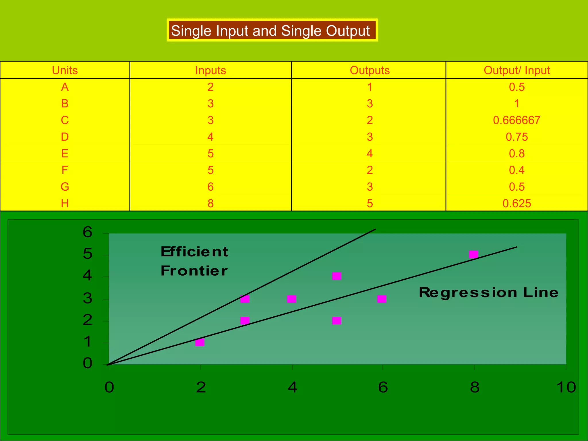
Analysis of efficiency metrics using a single input-output model, showcasing outputs divided by inputs.
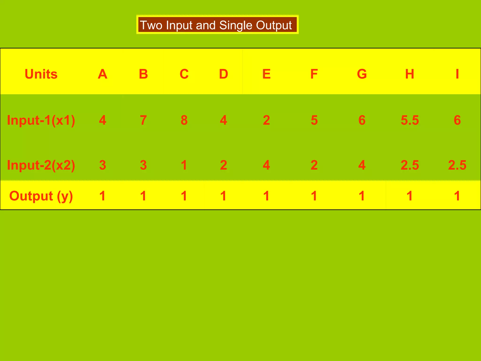
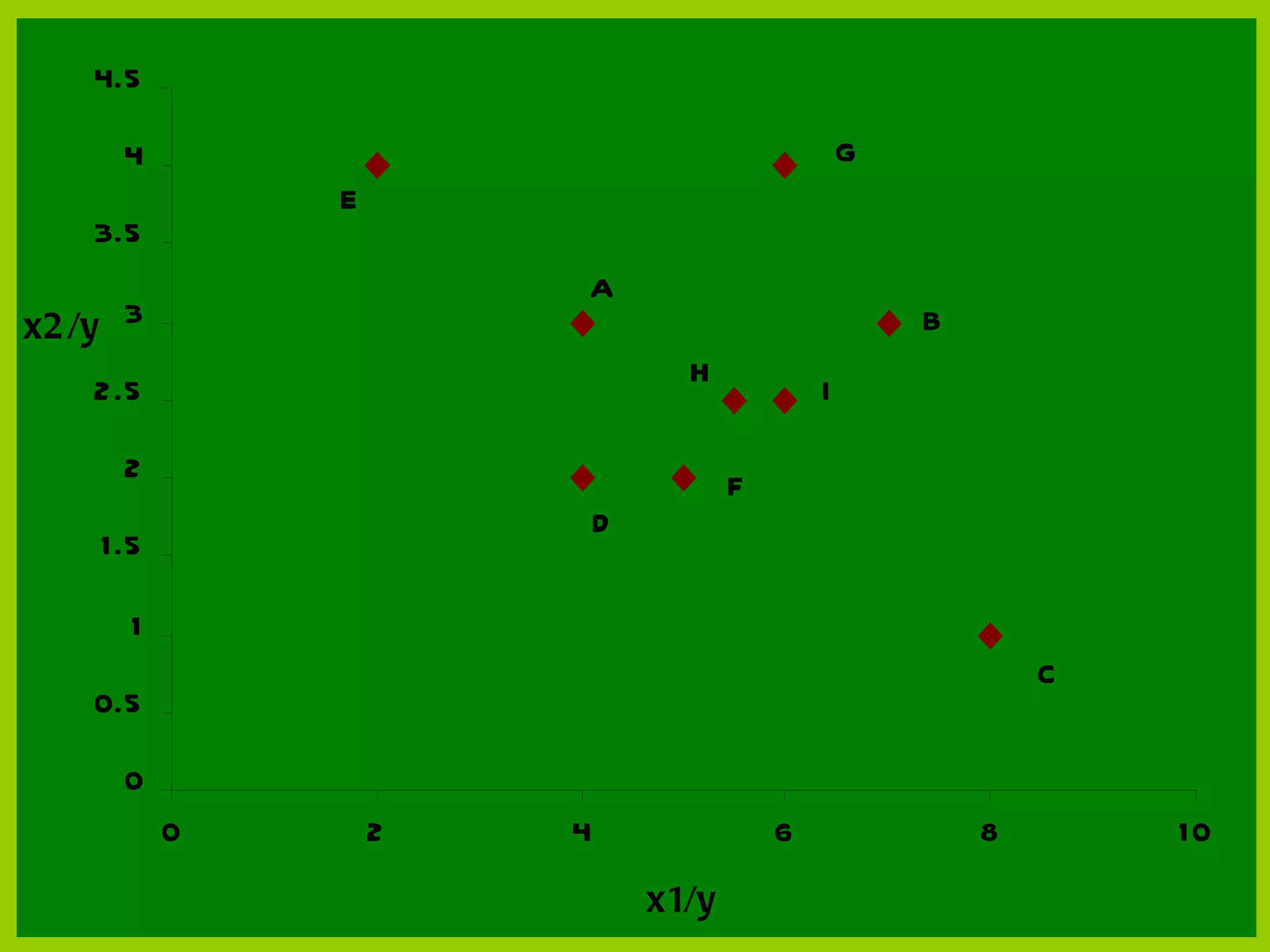
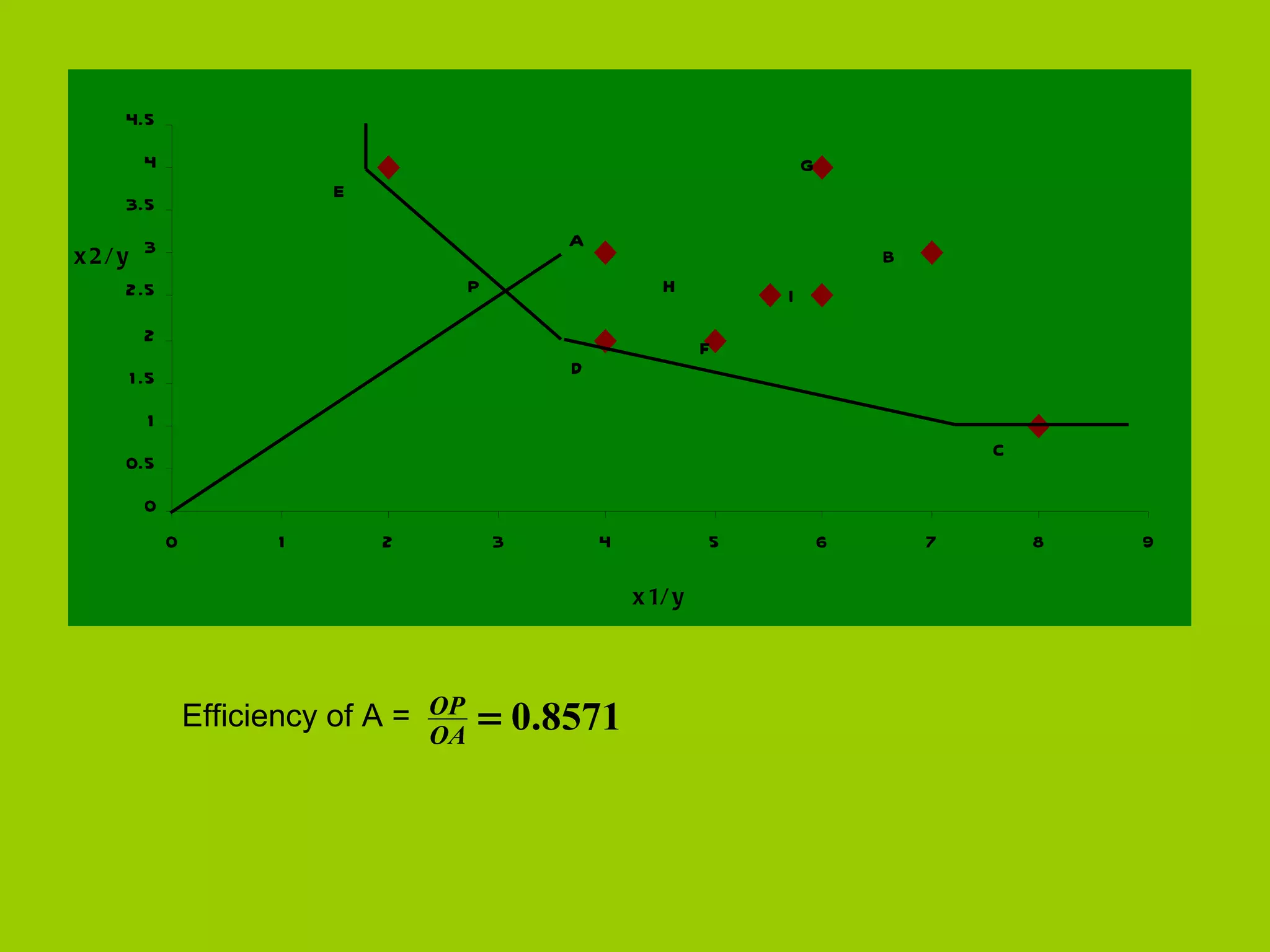
Efficiency calculated for units with multiple inputs and a single output, highlighting improvement of efficiency.
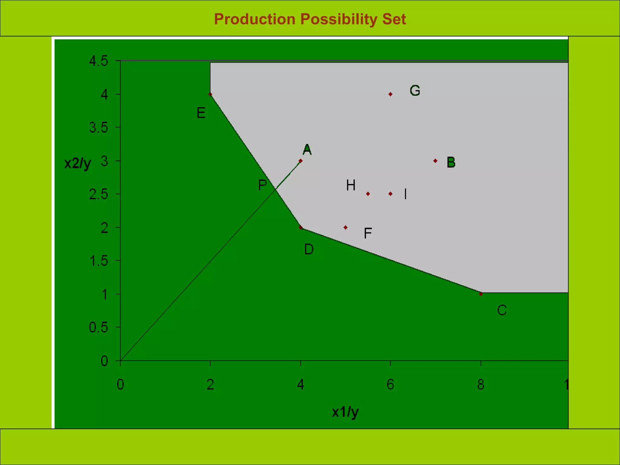
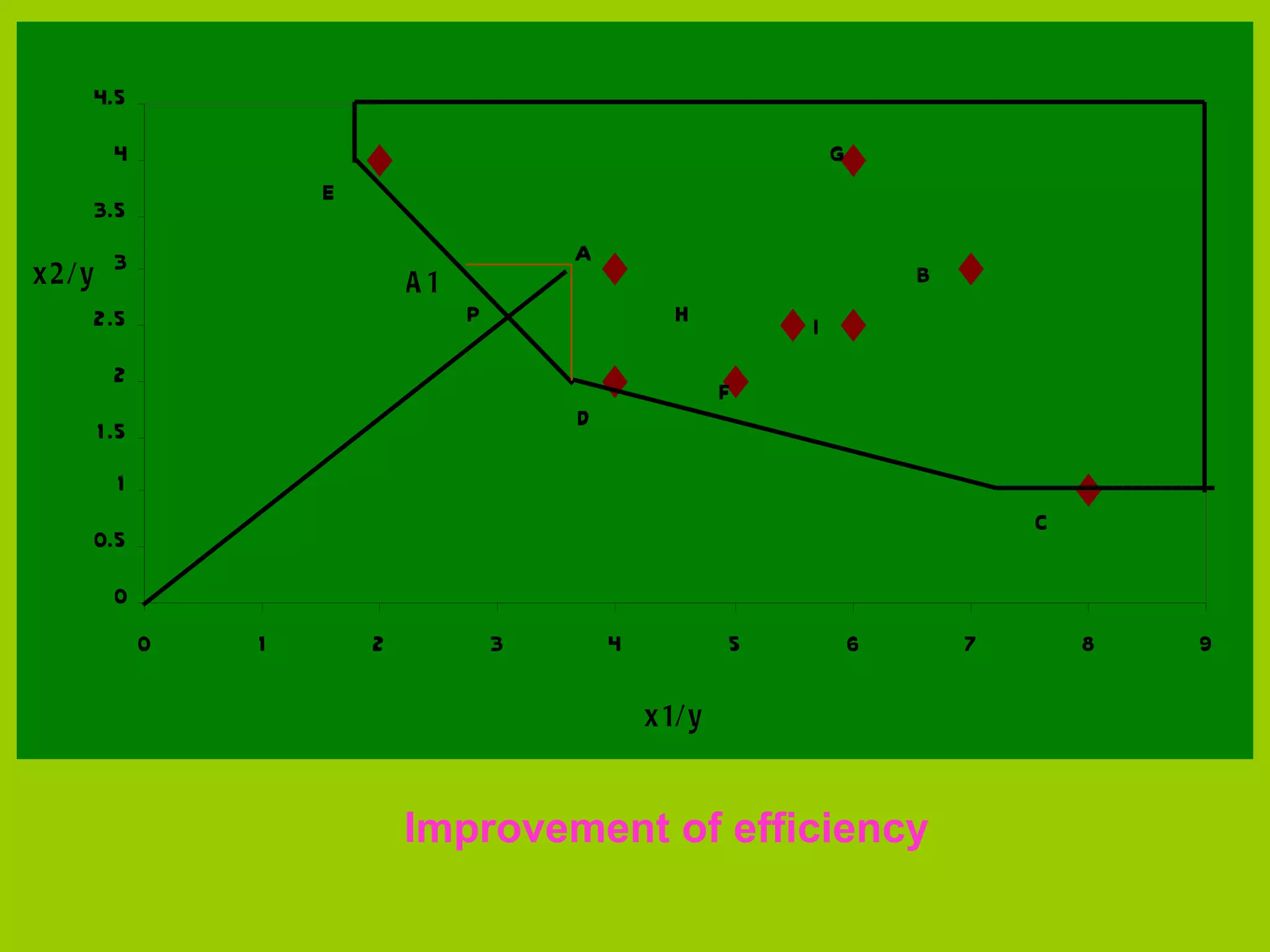
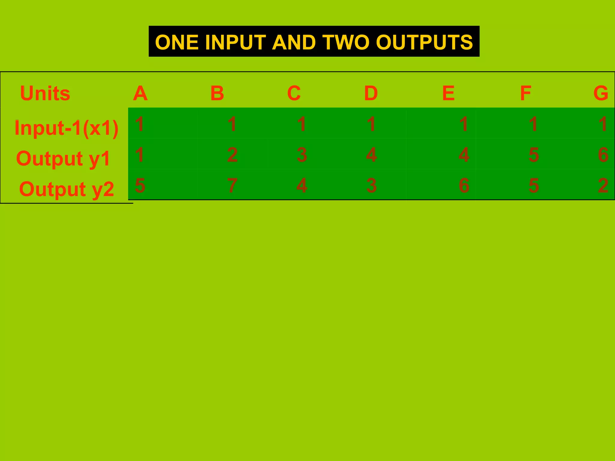
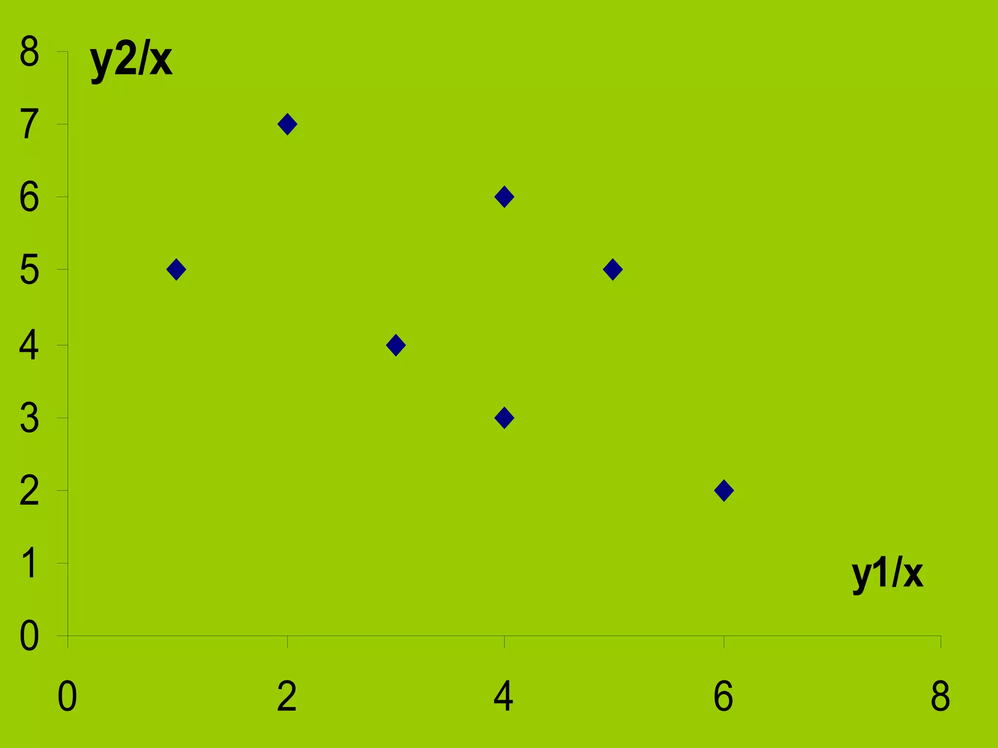
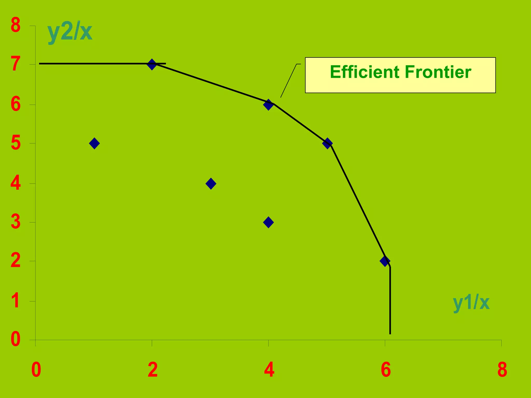
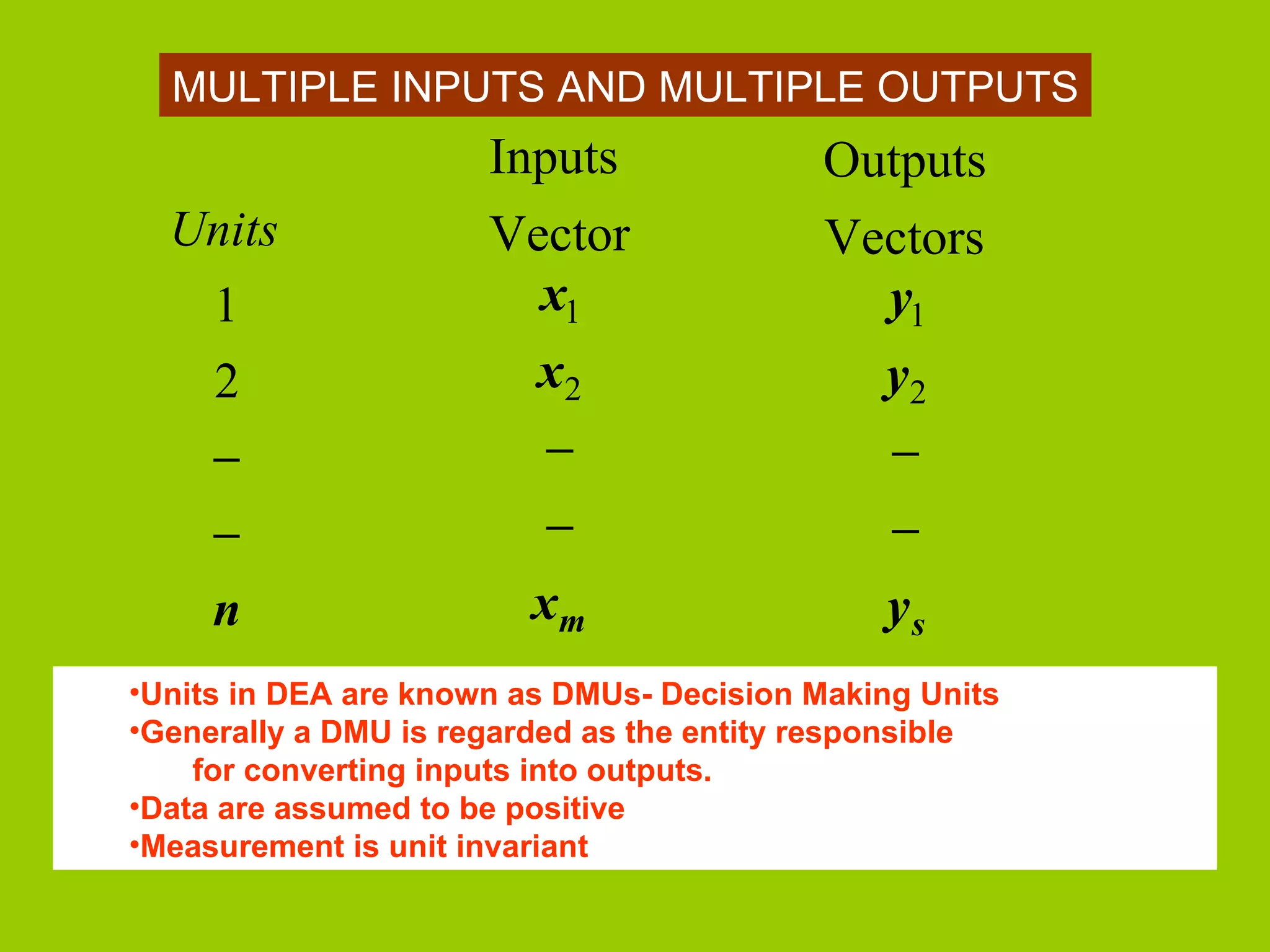
DEA framework where one input generates two outputs, with visual representation of efficiency frontiers.
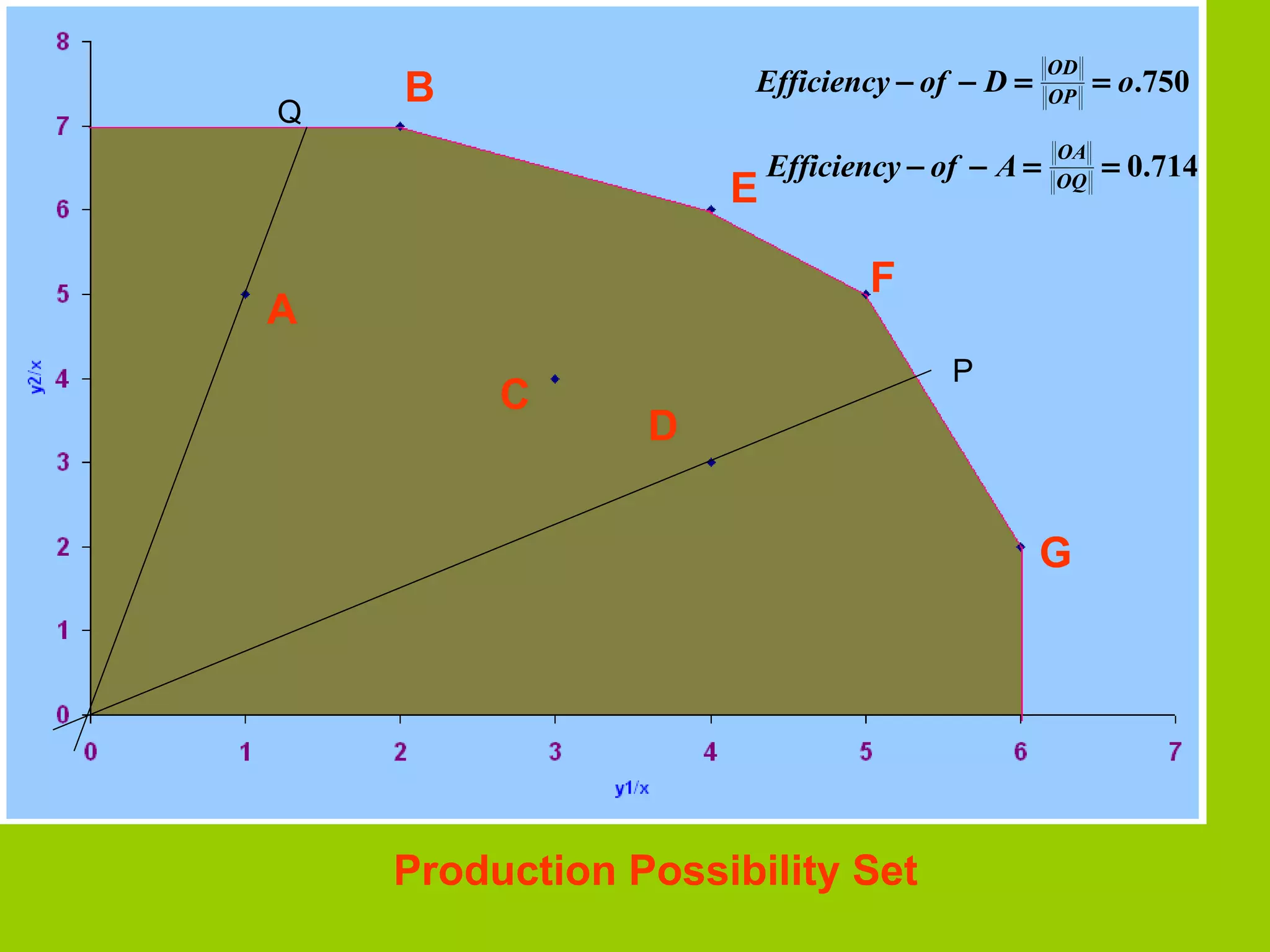
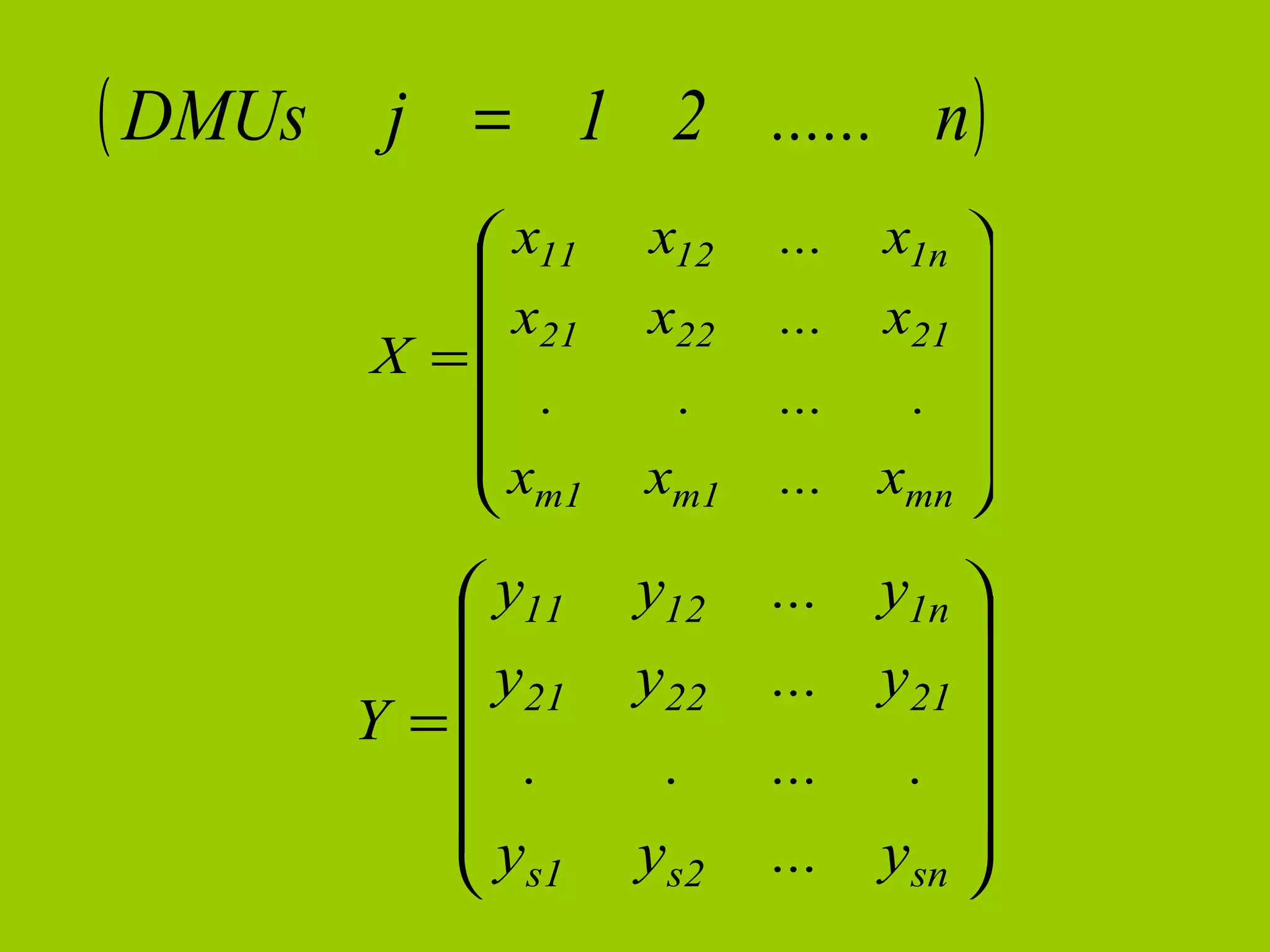
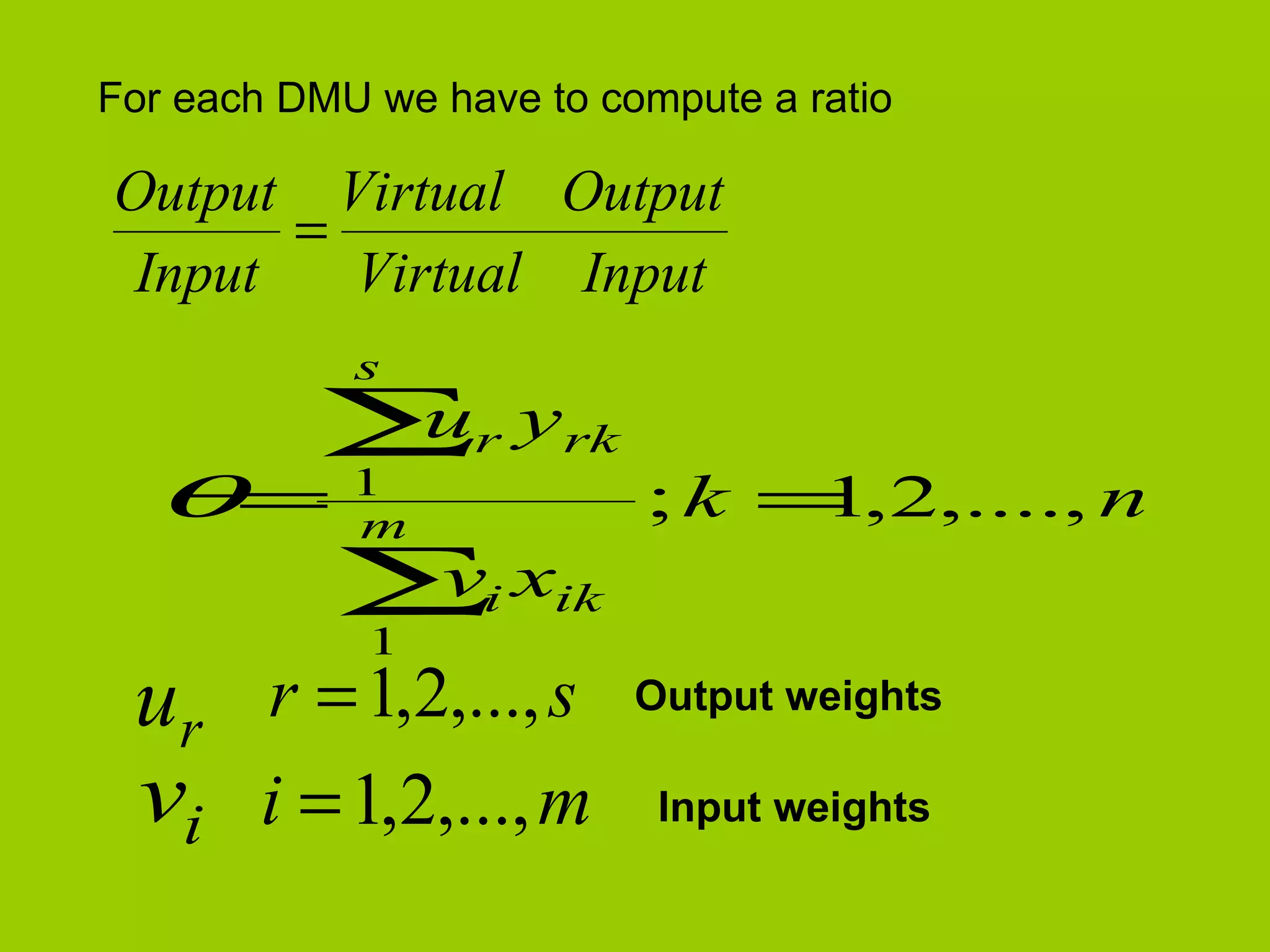
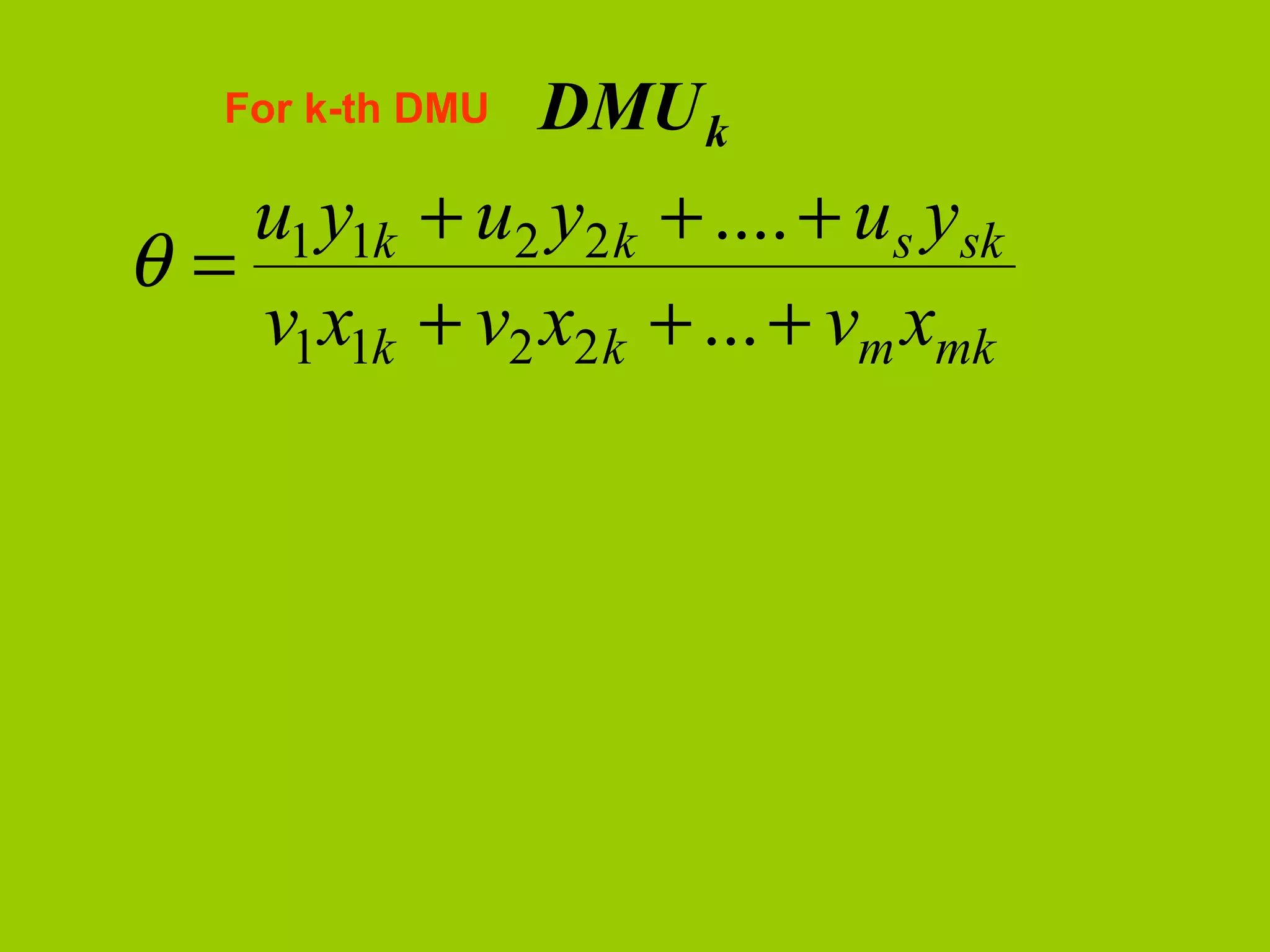
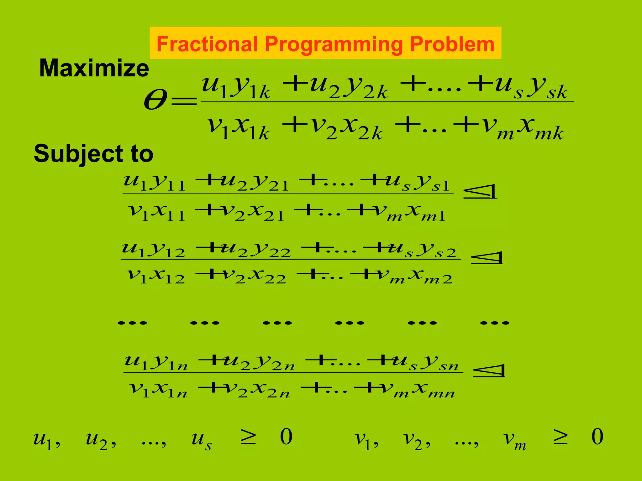
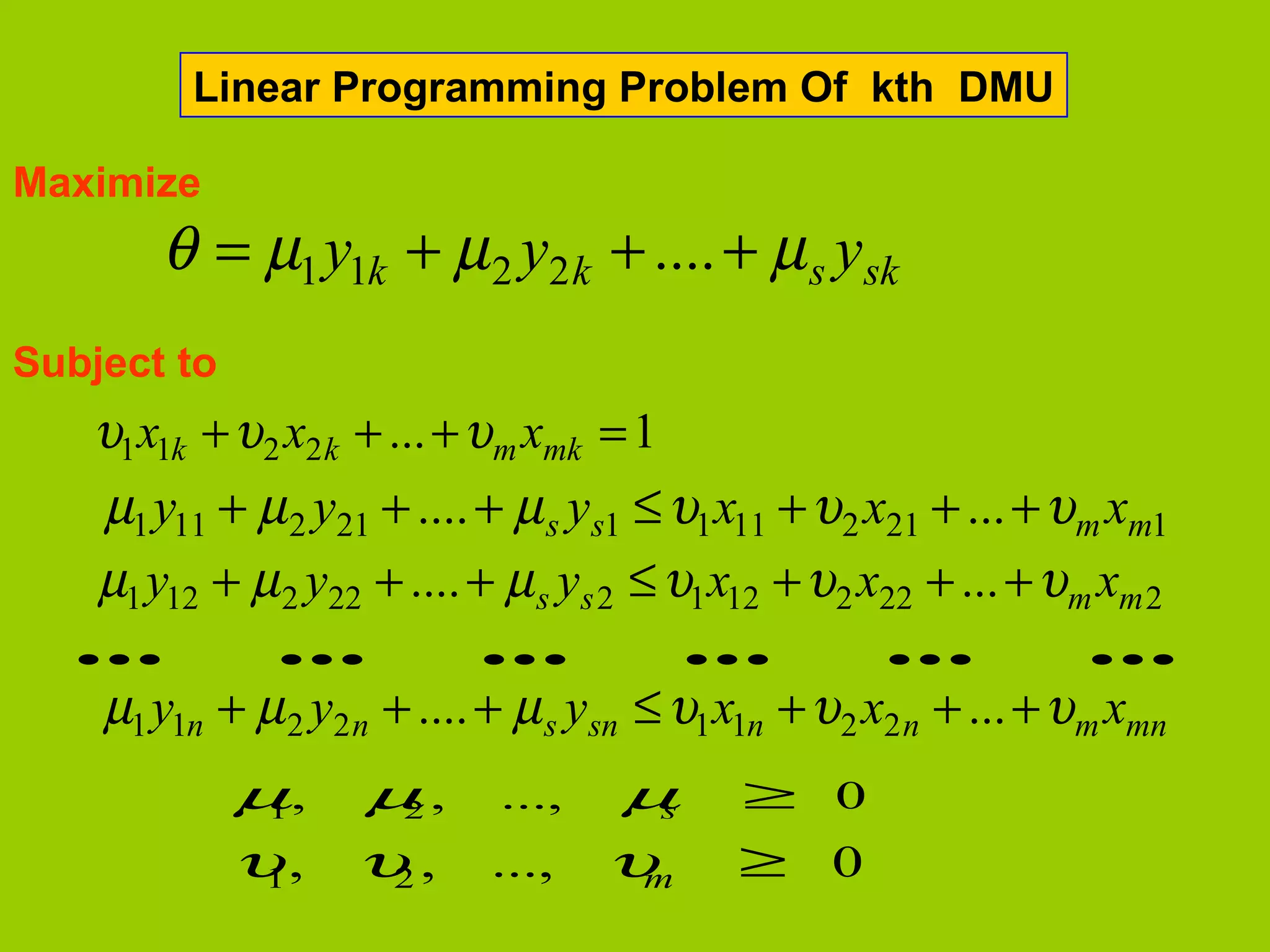
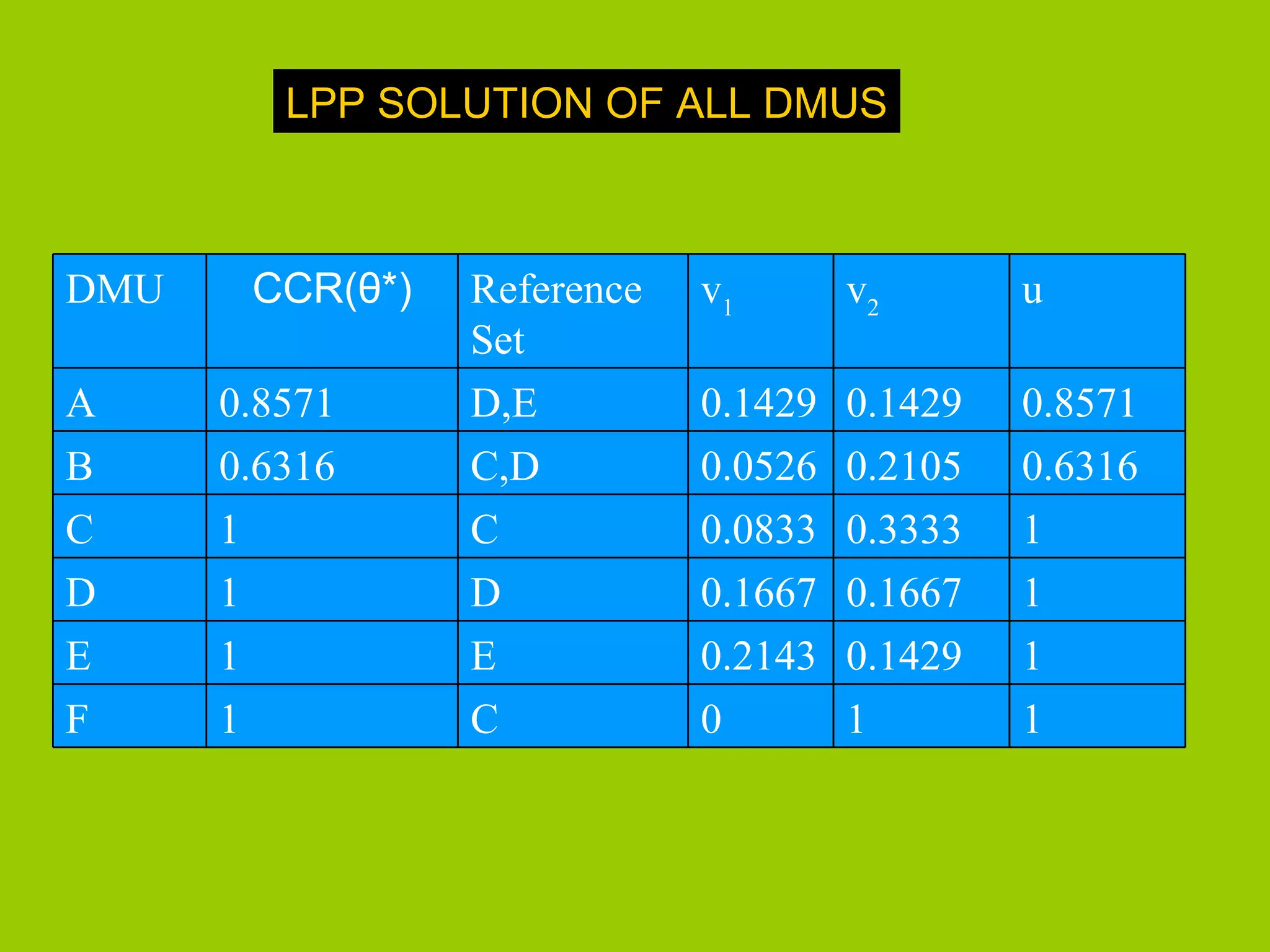
Calculating efficiency ratios of various Decision Making Units (DMUs) using a linear programming approach.
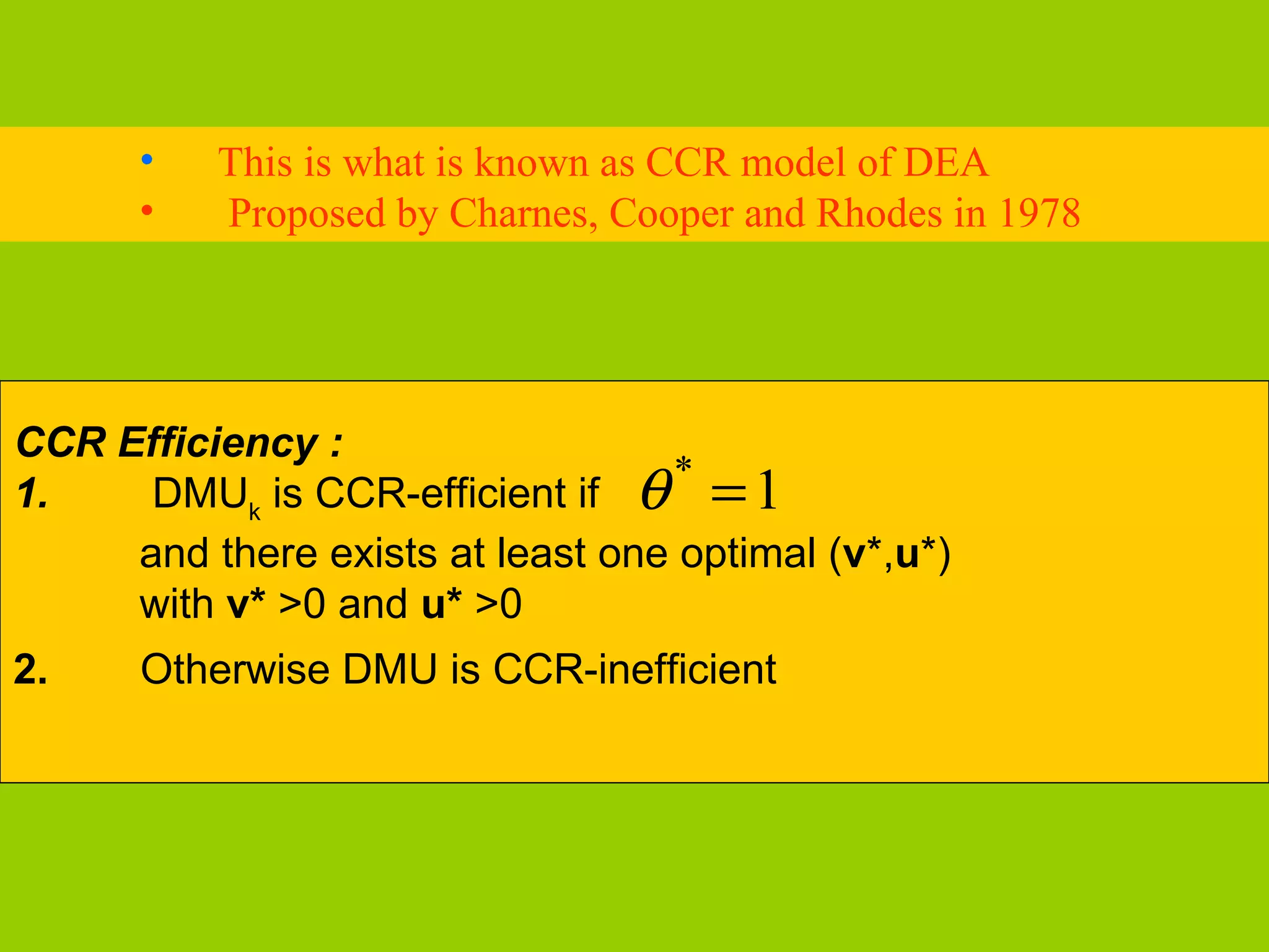
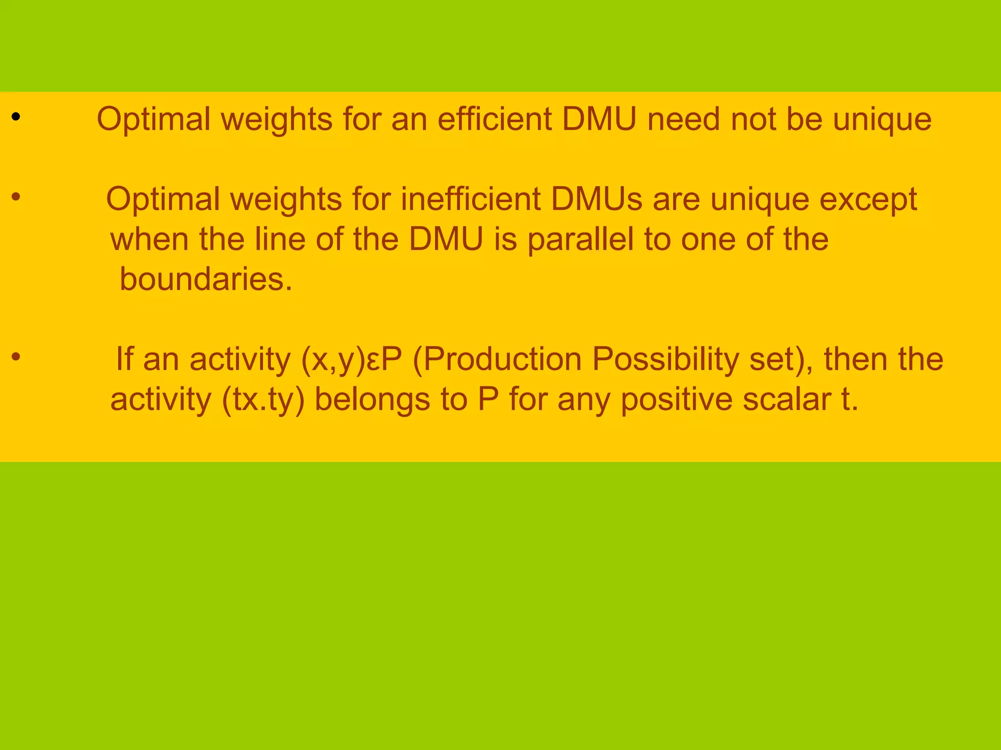
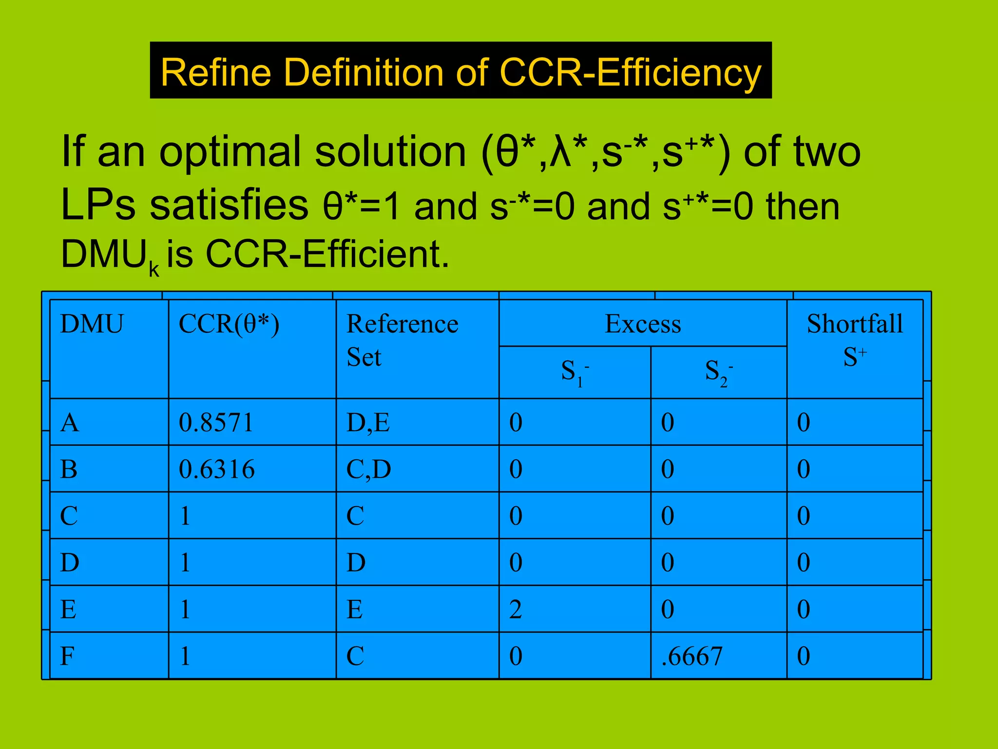
Details on the CCR model including conditions for DMU efficiency, optimal solutions, and proposed by Charnes et al.
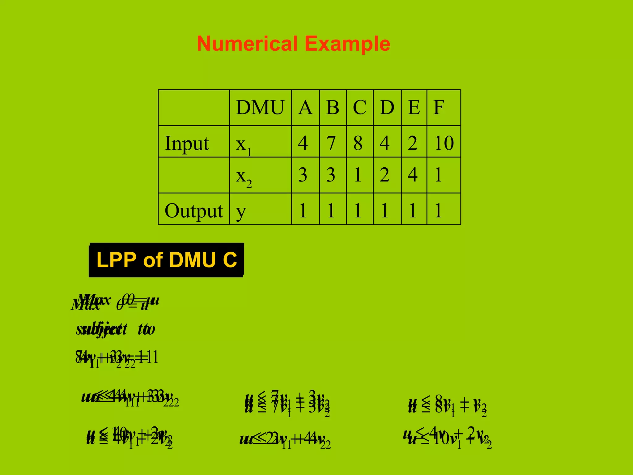
Numerical example evaluating DMU efficiency with focus on input-output ratios and computational solutions.
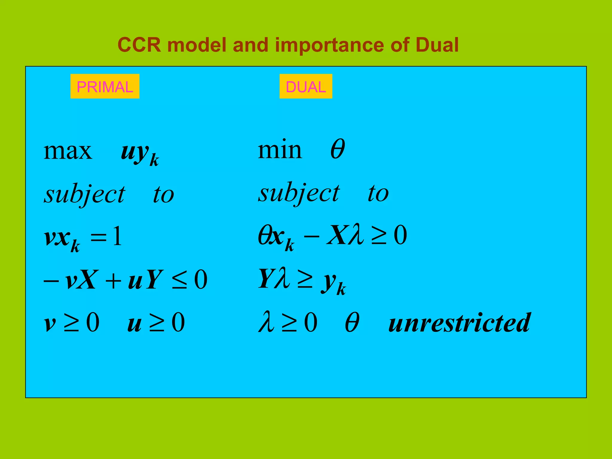
Discussion of primal and dual models within the CCR framework, emphasizing input and output relationship.
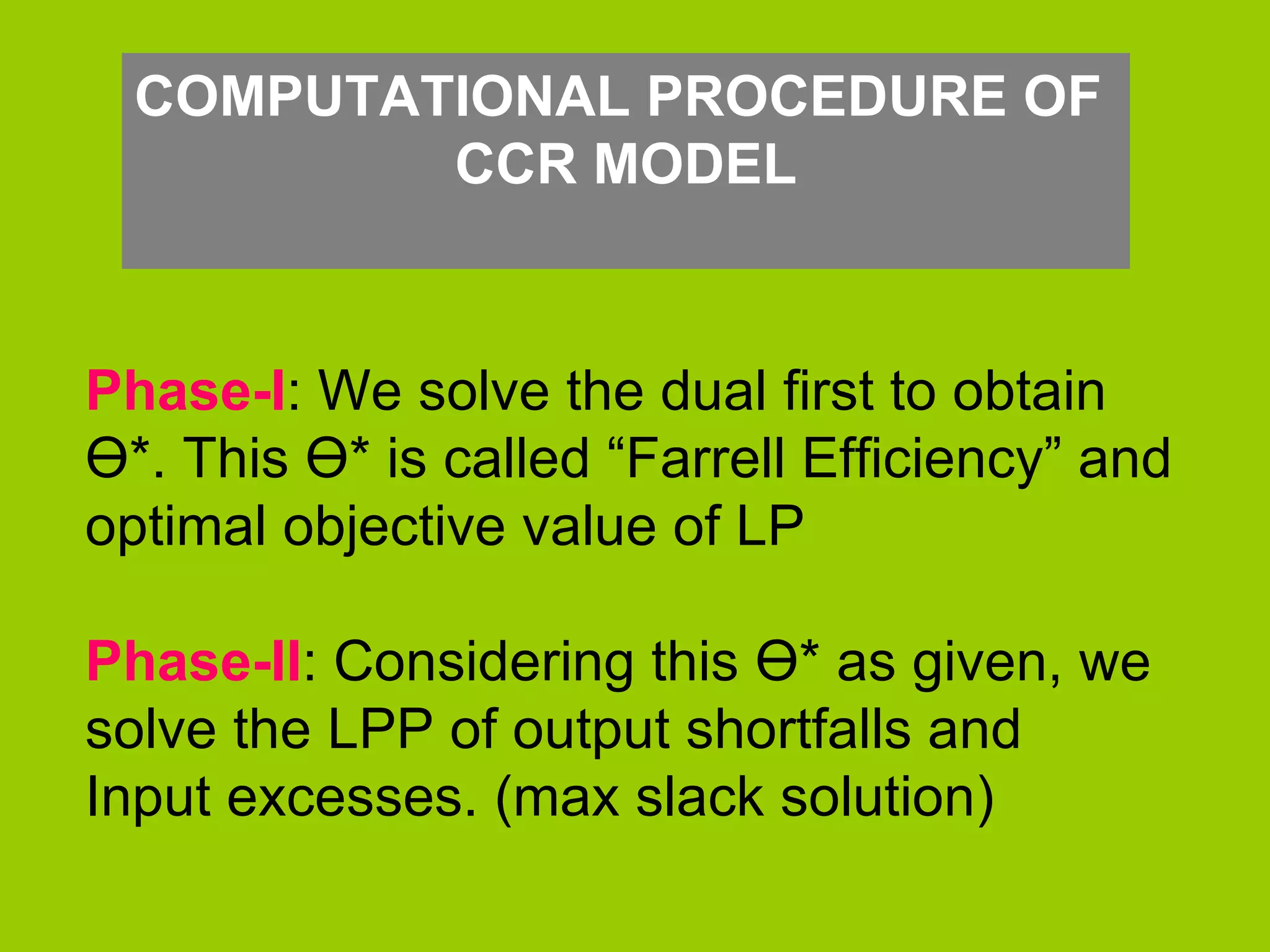
Steps involved in solving the CCR model to determine efficiency through dual solutions and slacks.
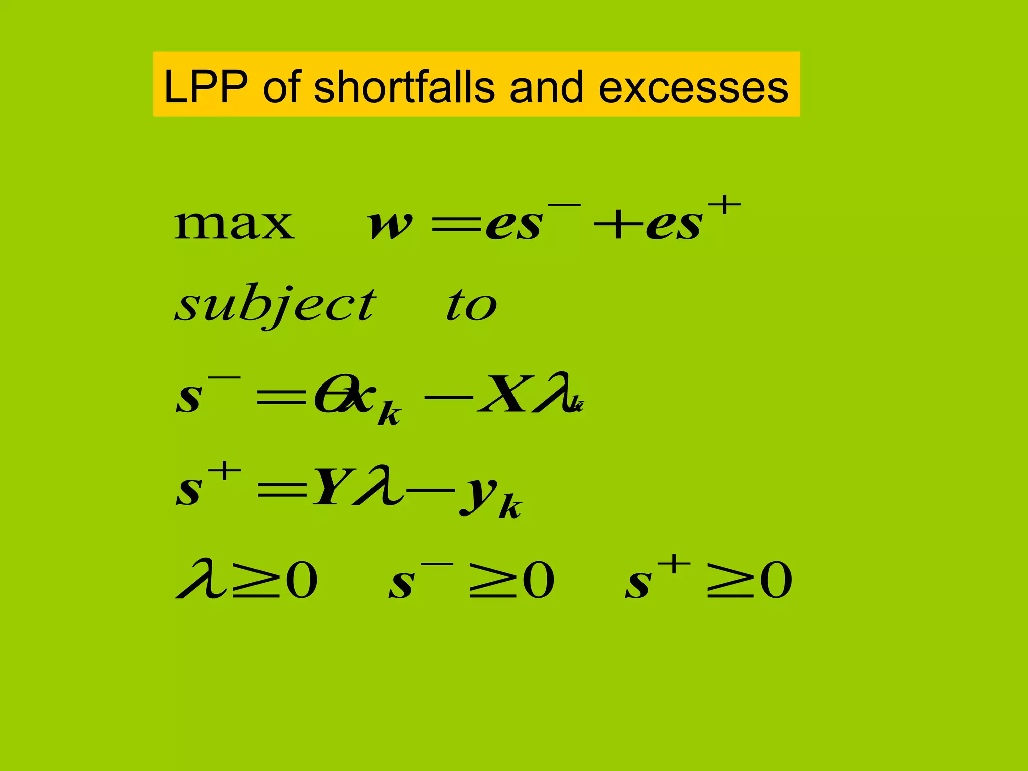
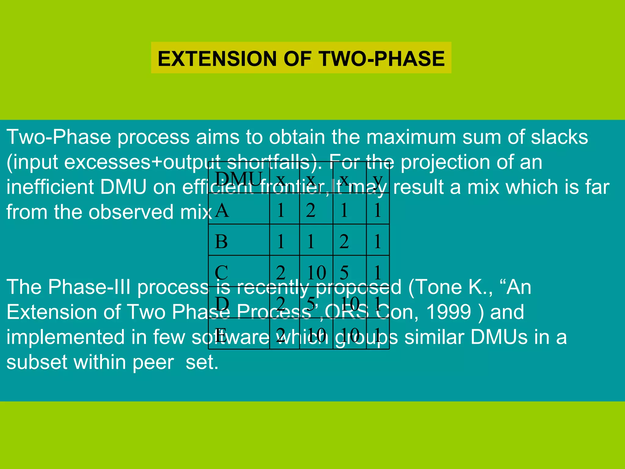
Extension for efficiency improvement through a two-phase model, leading to maximum slacks analysis.
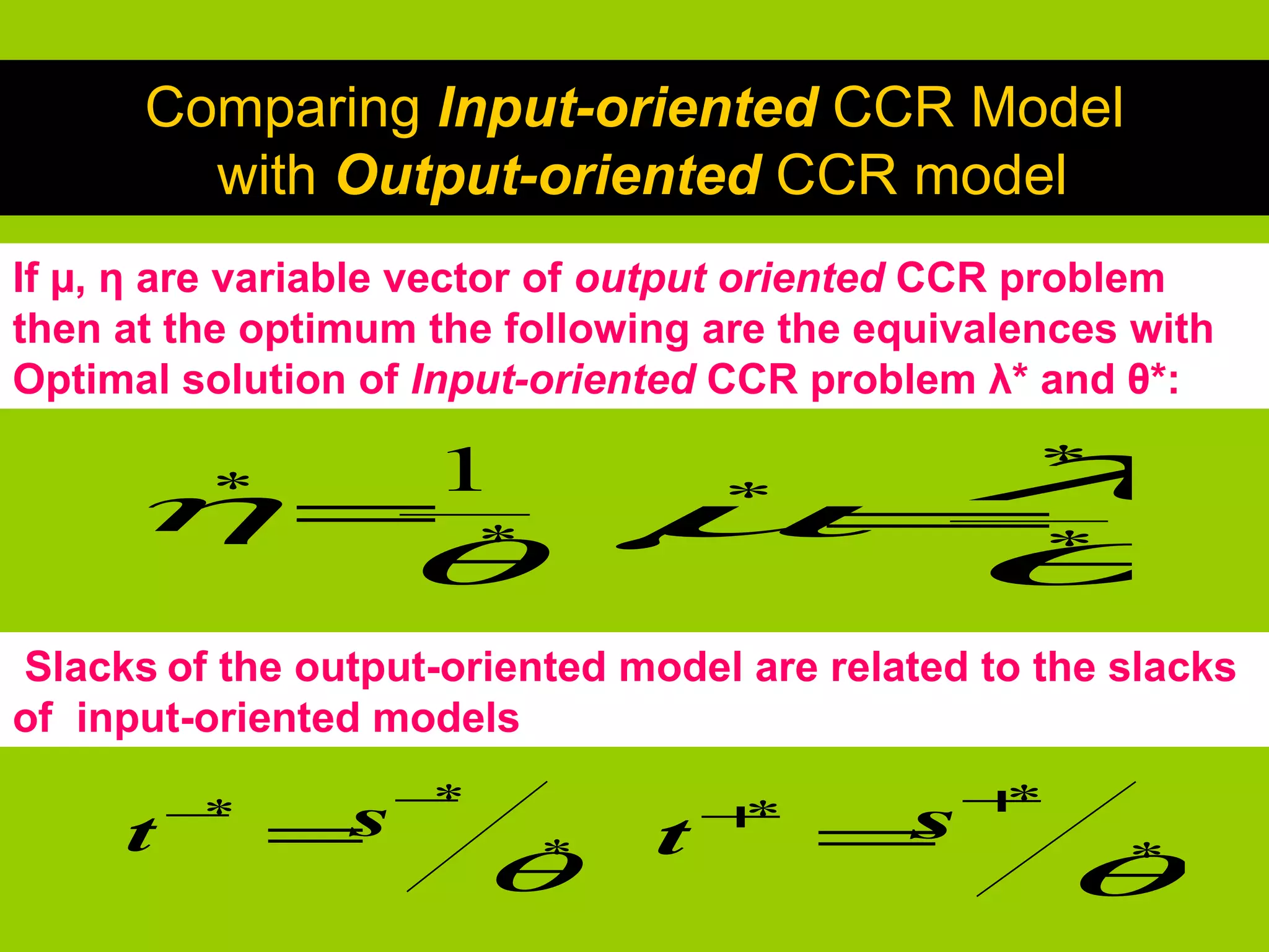
Comparison of input-oriented and output-oriented models, examining efficiencies across different DMUs.
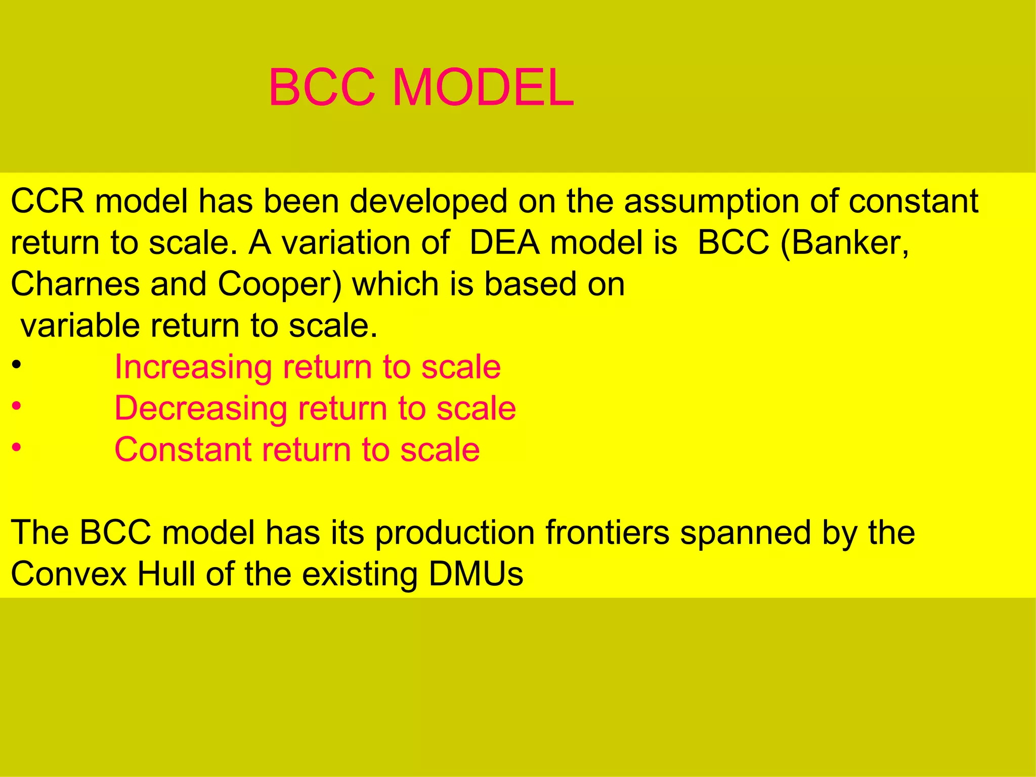
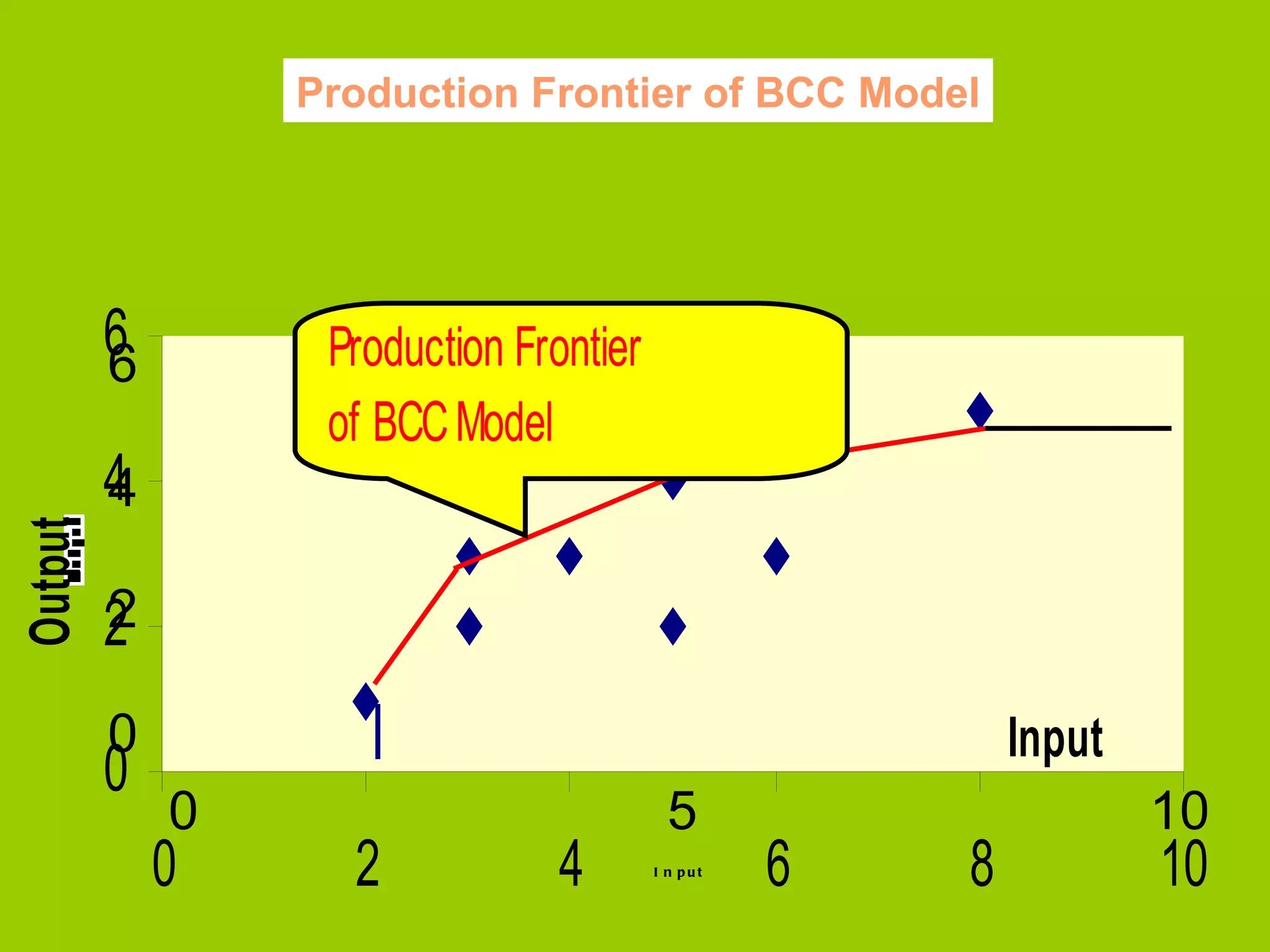
Introduction to the BCC model, which allows for variable returns to scale, and acknowledgment of resources.