The document discusses algorithm analysis and asymptotic notation. It introduces algorithms for computing prefix averages of an array in quadratic and linear time. Specifically:
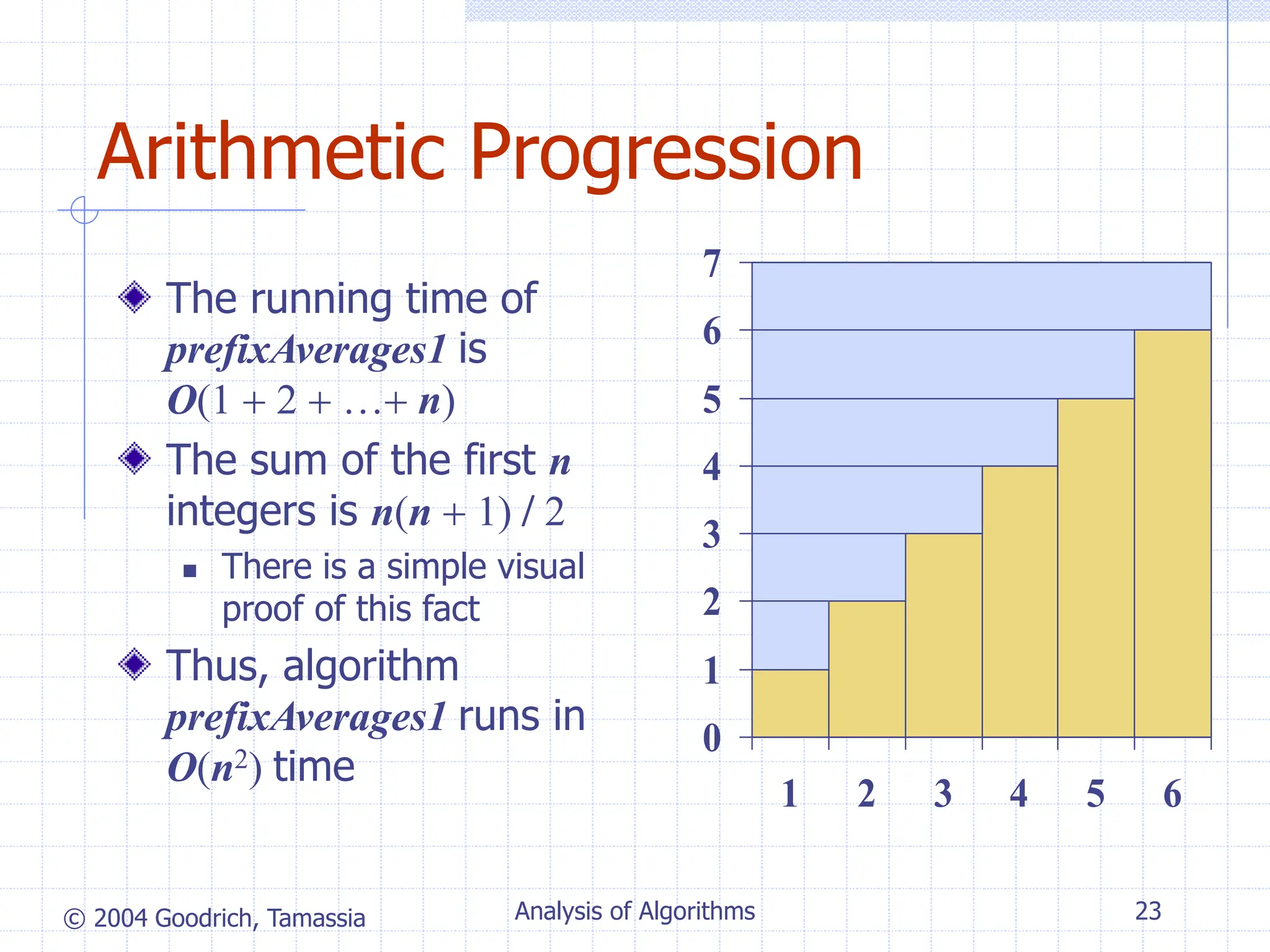
- An algorithm that computes prefix averages by directly applying the definition runs in O(n^2) time as its inner loop iterates over i elements n times.
- A more efficient algorithm that maintains a running sum runs in O(n) time, as each of its n iterations performs a constant number of operations.
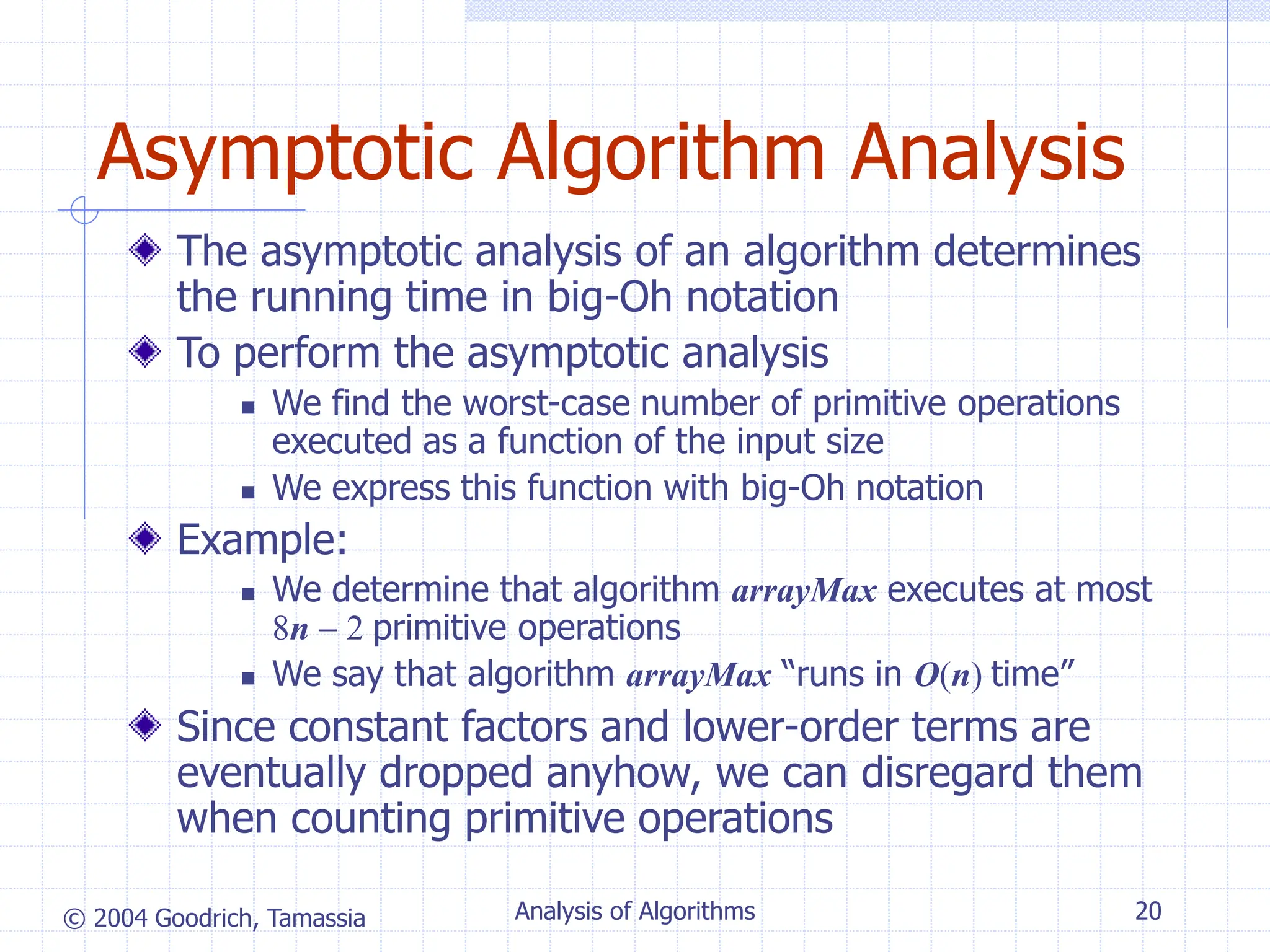
- Asymptotic analysis allows algorithms to be classified based on growth rate, ignoring constant factors. This provides an algorithm-independent analysis of computational complexity.
![© 2004 Goodrich, Tamassia Analysis of Algorithms 6
Pseudocode (§3.2)
High-level description
of an algorithm
More structured than
English prose
Less detailed than a
program
Preferred notation for
describing algorithms
Hides program design
issues
Algorithm arrayMax(A, n)
Input array A of n integers
Output maximum element of A
currentMax A[0]
for i 1 to n 1 do
if A[i] currentMax then
currentMax A[i]
return currentMax
Example: find max
element of an array](https://image.slidesharecdn.com/lec7-231222135518-c75a9b1d/75/analysis-of-algorithms-6-2048.jpg)
![© 2004 Goodrich, Tamassia Analysis of Algorithms 7
Pseudocode Details
Control flow
if … then … [else …]
while … do …
repeat … until …
for … do …
Indentation replaces braces
Method declaration
Algorithm method (arg [, arg…])
Input …
Output …
Method call
var.method (arg [, arg…])
Return value
return expression
Expressions
Assignment
(like in Java)
Equality testing
(like in Java)
n2 Superscripts and other
mathematical
formatting allowed](https://image.slidesharecdn.com/lec7-231222135518-c75a9b1d/75/analysis-of-algorithms-7-2048.jpg)
![© 2004 Goodrich, Tamassia Analysis of Algorithms 10
Counting Primitive
Operations (§3.4)
By inspecting the pseudocode, we can determine the
maximum number of primitive operations executed by
an algorithm, as a function of the input size
Algorithm arrayMax(A, n) # operations
currentMax A[0] 2
for i 1 to n 1 do 2n
if A[i] currentMax then 2(n 1)
currentMax A[i] 2(n 1)
{ increment counter i } 2(n 1)
return currentMax 1
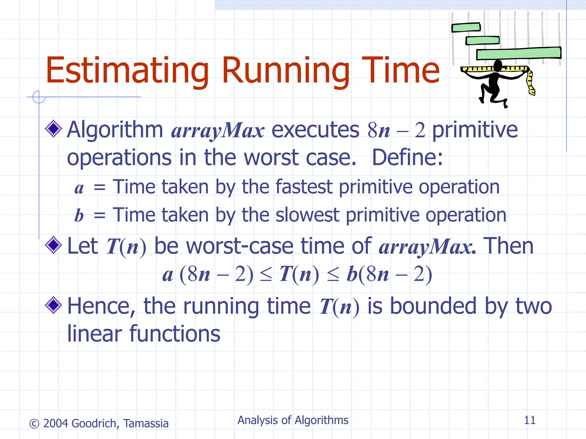
Total 8n 2](https://image.slidesharecdn.com/lec7-231222135518-c75a9b1d/75/analysis-of-algorithms-10-2048.jpg)
![© 2004 Goodrich, Tamassia Analysis of Algorithms 21
Computing Prefix Averages
We further illustrate
asymptotic analysis with
two algorithms for prefix
averages
The i-th prefix average of
an array X is average of the
first (i + 1) elements of X:
A[i] (X[0] + X[1] + … + X[i])/(i+1)
Computing the array A of
prefix averages of another
array X has applications to
financial analysis
0
5
10
15
20
25
30
35
1 2 3 4 5 6 7
X
A](https://image.slidesharecdn.com/lec7-231222135518-c75a9b1d/75/analysis-of-algorithms-21-2048.jpg)
![© 2004 Goodrich, Tamassia Analysis of Algorithms 22
Prefix Averages (Quadratic)
The following algorithm computes prefix averages in
quadratic time by applying the definition
Algorithm prefixAverages1(X, n)
Input array X of n integers
Output array A of prefix averages of X #operations
A new array of n integers n
for i 0 to n 1 do n
s X[0] n
for j 1 to i do 1 + 2 + …+ (n 1)
s s + X[j] 1 + 2 + …+ (n 1)
A[i] s / (i + 1) n
return A 1](https://image.slidesharecdn.com/lec7-231222135518-c75a9b1d/75/analysis-of-algorithms-22-2048.jpg)
![© 2004 Goodrich, Tamassia Analysis of Algorithms 24
Prefix Averages (Linear)
The following algorithm computes prefix averages in
linear time by keeping a running sum
Algorithm prefixAverages2(X, n)
Input array X of n integers
Output array A of prefix averages of X #operations
A new array of n integers n
s 0 1
for i 0 to n 1 do n
s s + X[i] n
A[i] s / (i + 1) n
return A 1
Algorithm prefixAverages2 runs in O(n) time](https://image.slidesharecdn.com/lec7-231222135518-c75a9b1d/75/analysis-of-algorithms-24-2048.jpg)