An introduction on normalizing flows

An introduction to Normalizing Flows
Grigorios Chrysos
École polytechnique fédérale de Lausanne
January 19, 2021
Grigorios Chrysos An introduction to Normalizing Flows January 19, 2021 1 / 26

1 Introduction to Normalizing Flows
2 Taxonomy of Normalizing Flows
3 Practical considerations and limitations
4 Analyzing inverse problems
5 Generative modeling with Glow

Goal of normalizing flows
Data space X Latent space Z
Inference
x ∼ p̂X
z = f (x)
⇒
Generation
z ∼ pZ
x = f −1
(z)
⇐
Figure: Perform both mappings with a single network.
Dinh, Laurent, Jascha Sohl-Dickstein, and Samy Bengio. ”Density estimation using real nvp.”, International Conference on
Learning Representations (ICLR) 2017.

Formulation
Suppose we want to define a joint distribution over x ∈ RD.
Idea: Express x as a transformation f of a real vector u sampled from
pu(u):
x = f (u) with u ∼ pu(u) (1)
The transformation f must be invertible1 and both f and f −1 must
be differentiable.
1
Normalizing flows are often referred to as ‘Invertible neural networks’.

Formulation
Then, using the change of variables:
px (x) = pu(u)|Jf (u)|−1
(2)
where | · | denotes the determinant and Jf the Jacobian matrix.
The Jacobian Jf is a D × D matrix; it is crucial to define a
transformation that has an easy-to-compute Jacobian (or its inverse).
The term |Jf (u)| is the relative change of volume in a small
neighborhood around u.

Properties
Compositionality of fi : the composition of the two transformations f1
and f2 is denoted as f2 ◦ f1 and has:
|Jf2◦f1 (u)| = |Jf2 (f1(u))| · |Jf1 (u)| (3)
Expressive power: INNs can approximate any distribution px (x) under
mild conditions.

Taxonomy
The normalizing flows are categorized as follows (Kobyzev, 2020):
Elementwise bijections.
Linear flows.
Coupling and autoregressive flows.
Residual flows.
Continuous-time flows2.
Kobyzev, Ivan, Simon Prince, and Marcus Brubaker. “Normalizing flows: An introduction and review of current methods.” IEEE
Transactions on Pattern Analysis and Machine Intelligence (2020).
2
Not covered in this presentation; included for thoroughness.

Elementwise bijections
Let gθ : R → R be a bijective function, θ are (learnable) parameters
and x = (x1, . . . , xD)T .
Then, f (x) = (gθ(x1), . . . , gθ(xD))T is a bijection.
A different bijective function gθi
can be applied to each element xi .
Leaky RELU, or Softplus are two types of elementwise bijections.
Drawback: No correlation between different elements.

Linear flows
Let Aθ ∈ RD×D an invertible matrix.
The linear transformation f (x) = Aθx captures correlations between
dimensions.
The following forms of Aθ have been used: diagonal, triangular, LU
decomposition, permutation matrix.
Drawback: Limited expressivity.

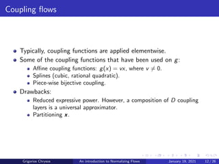
Coupling flows
Let xA ∈ Rd and xB ∈ RD−d two disjoint partitions of x. Let
g : Rd → Rd be a bijective function, and φθ any arbitrary function.
The coupling flow realizes the mapping:
uA = g(xA, φθ(xB)), uB = xB (4)
where u = [uA, uB] is the output of the coupling layer.
The inverse of the coupling flow exists only if g is invertible. Then,
the inverse is:
xA = g−1
(uA, φθ(xB)), xB = uB (5)

Coupling flows
Typically, coupling functions are applied elementwise.
Some of the coupling functions that have been used on g:
Affine coupling functions: g(x) = vx, where v 6= 0.
Splines (cubic, rational quadratic).
Piece-wise bijective coupling.
Drawbacks:
Reduced expressive power. However, a composition of D coupling
layers is a universal approximator.
Partitioning x.

Autoregressive flows
Let gn : R → R be a bijective function with (learnable) parameters n.
The autoregressive flow is ut = gn (xt, φθ(x1:t−1)), where
x1:t = (x1, . . . , xt).
The Jacobian is triangular, however the computation of the inverse is
challenging.
Drawbacks:
Flow dependent on the order of the input variables.
Sequential computation; hard to parallelize.

Residual flows
The flow is u = x + gθ(x).
Invertible only when gθ is constrained appropriately3.
Planar and radial flows are special cases of the residual flow:
Planar flow: f (x) = x + vg(wT
x + b), where g is a smooth,
elementwise non-linearity, v, w ∈ RD
.
Radial flow: f (x) = x + β/(a + ||x − x0||), where x0 is a selected point.
3
For instance, the block is invertible when the Lipschitz constant of the residual
block is smaller than 1.

Practical considerations
Batch normalization has a diagonal Jacobian, so it can be used as a
transformation.
Linear transformations are often combined with other flows: coupling
layers are often used in conjunction with permutation.
A series of flows are typically learned:
x f1
←→ h1
f2
←→ h2
f3
←→ . . .
fN
←→ u.

Limitations
Computational efficiency; for instance, GLOW (Kingma, 2018) uses
∼ 200M parameters and ∼ 600 convolution layers.
Inductive bias: modeling the invertible transformations.
Normalizing flows for non-Euclidean spaces.
Flows for discrete random variables.
Kingma, Durk P., and Prafulla Dhariwal. “Glow: Generative flow with invertible 1x1 convolutions.” In Advances in neural
information processing systems, pp. 10215-10224. 2018.

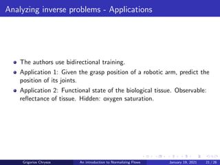
Analyzing inverse problems
Let y ∈ RM be a measurement and x ∈ RD be the hidden variable in
the forward process y = s(x) with M < D.
Let z ∈ RK be a latent random variable, such that we want to learn a
function g with [y, z] = g(x).
Ardizzone, Lynton, Jakob Kruse, Sebastian Wirkert, Daniel Rahner, Eric W. Pellegrini, Ralf S. Klessen, Lena Maier-Hein,
Carsten Rother, and Ullrich Köthe. “Analyzing inverse problems with invertible neural networks.” ICLR 2019.

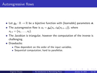
Analyzing inverse problems - Coupling layers
They define the following coupling layers with inputs [uA, uB]:
vA = uA

exp(sA(vA))+tA(vA) (6)
The inverse can be easily defined given inputs [vA, vB]:
uB = (vB−tA(vA))

exp(−sA(vA)), uA = (vA−tB(uB))

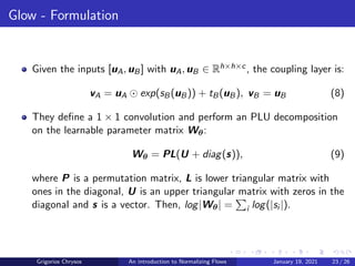
is an elementwise product, and si , ti , i ∈ [A, B] can have
learnable parameters.

Analyzing inverse problems - Applications
The authors use bidirectional training.
Application 1: Given the grasp position of a robotic arm, predict the
position of its joints.
Application 2: Functional state of the biological tissue. Observable:
reflectance of tissue. Hidden: oxygen saturation.

An introduction on normalizing flows

More Related Content

What's hot

Similar to An introduction on normalizing flows

Recently uploaded

An introduction on normalizing flows