Download as PDF, PPTX

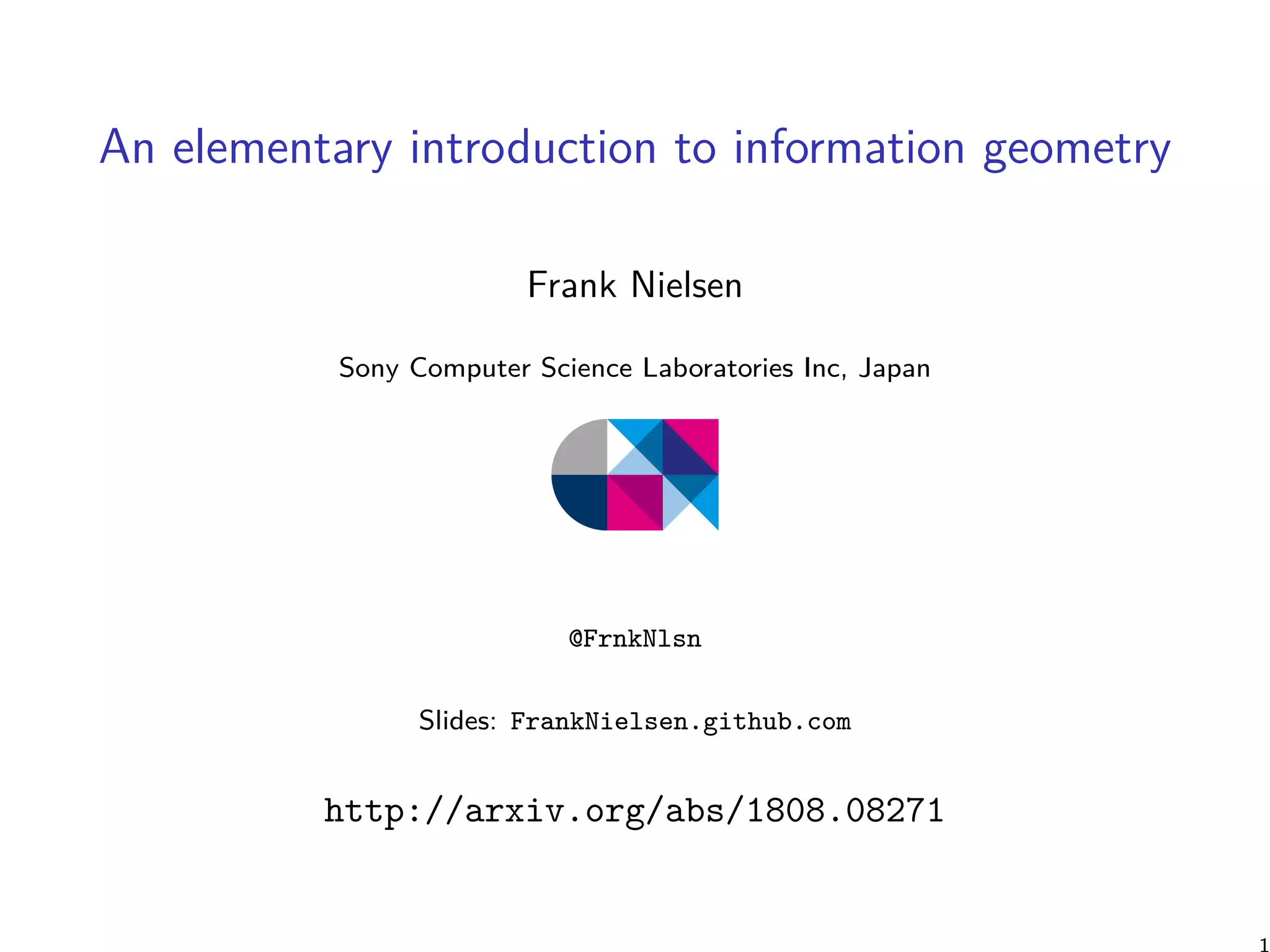
![Fundamental theorem of Riemannian geometry
Theorem (Levi-Civita connection from metric tensor)
There exists a unique torsion-free affine connection compatible with the
metric called the Levi-Civita connection: LC∇
Christoffel symbols of the Levi-Civita connection can be expressed
from the metric tensor
LC
Γk
ij
Σ
=
1
2
gkl
(∂igil + ∂jgil − ∂lgij)
where gij denote the matrix elements of the inverse matrix g−1.
“Geometric” equation defining the Levi-Civita connection is given by
the Koszul formula:
2g(∇XY, Z) = X(g(Y, Z)) + Y(g(X, Z)) − Z(g(X, Y))
+ g([X, Y], Z) − g([X, Z], Y) − g([Y, Z], X).](https://image.slidesharecdn.com/introig-inriaoct2-2018-181004165425/85/An-elementary-introduction-to-information-geometry-15-320.jpg)
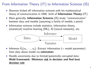
![Curvature tensor R of an affine connection ∇
Riemann-Christoffel 4D curvature tensor R (Ri
jkl):
Geometric equation:
R(X, Y)Z = ∇X∇YX − ∇Y∇XZ − ∇[X,Y]Z
where [X, Y](f) = X(Y(f)) − Y(X(f)) (∀f ∈ F(M)) is the Lie bracket
of vector fields
Manifold is flat = ∇-flat (i.e., R = 0) when there exists a
coordinate system x such that Γk
ij(x) = 0, i.e., all connection
coefficients vanish
Manifold is torsion-free when connection is symmetric: Γk
ij = Γk
ji
Geometric equation:
∇XY − ∇YX = [X, Y]](https://image.slidesharecdn.com/introig-inriaoct2-2018-181004165425/85/An-elementary-introduction-to-information-geometry-16-320.jpg)
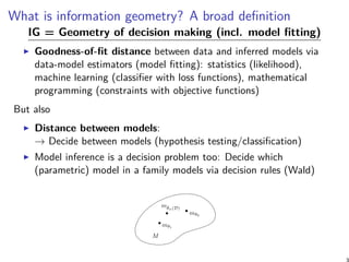
![Panorama of information-geometric structures
Riemannian Manifolds
(M, g) = (M, g, LC
)
Smooth Manifolds
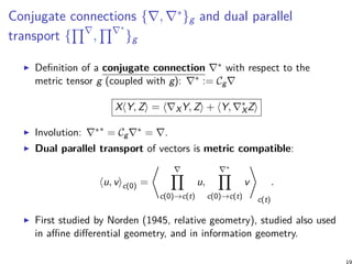
Conjugate Connection Manifolds
(M, g, , ∗
)
(M, g, C = Γ∗
− Γ)
Distance = Non-metric divergence Distance = Metric geodesic length
g = Fisher
g
Fisher
gij = E[∂il∂jl]
Spherical Manifold Hyperbolic Manifold
Self-dual Manifold
Dually flat Manifolds
(M, F, F∗
)
(Hessian Manifolds)
Dual Legendre potentials
Bregman Pythagorean theorem
Divergence Manifold
(M, Dg
, D
, D ∗
= D∗
)
D
− flat ⇔ D ∗
− flat
f-divergences Bregman divergence
Expected Manifold
(M, Fisher
g, −α
, α
)
α-geometry
Multinomial
family
LC
= + ∗
2
Euclidean Manifold
Location-scale
family
Location
family
Parametric
families
Fisher-Riemannian
Manifold
KL∗ on exponential families
KL on mixture families
Conformal divergences on deformed families
Etc.
Frank Nielsen
Cubic skewness tensor
Cijk = E[∂il∂jl∂kl]
αC = αFisher
g
α = 1+α
2
+ 1−α
2
∗
Γ±α = ¯Γ α
2
C(M, g, −α
, α
)
(M, g, αC)
canonical
divergence
I[pθ : p
θ
] = D(θ : θ )
Divergence D induces structure (M, Dg, D∇α, D∇−α) ≡ (M, Dg, DαC)
Convex potential F induces structure (M, Fg, F∇α, F∇−α) ≡ (M, Fg, FαC)
(via Bregman divergence BF)](https://image.slidesharecdn.com/introig-inriaoct2-2018-181004165425/85/An-elementary-introduction-to-information-geometry-22-320.jpg)
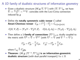
![Dually flat manifold
Consider a strictly convex smooth function F, called a potential
function
Associate its Bregman divergence (parameter divergence):
BF(θ : θ′
) := F(θ) − F(θ′
) − (θ − θ′
)⊤
∇F(θ′
)
The induced information-geometric structure is
(M, Fg, FC) := (M, BF g, BF C) with:
F
g := BF
g = −
[
∂i∂jBF(θ : θ′
)|θ′=θ
]
= ∇2
F(θ)
F
Γ := BF
Γijk(θ) = 0
F
Cijk := BF
Cijk = ∂i∂j∂kF(θ)
The manifold is F∇-flat
Levi-Civita connection LC∇ is obtained from the metric tensor Fg
(usually not flat), and we get the conjugate connection
(F∇)∗ = F∇−1 from (M, Fg, FC)](https://image.slidesharecdn.com/introig-inriaoct2-2018-181004165425/85/An-elementary-introduction-to-information-geometry-24-320.jpg)
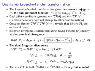
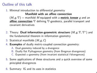
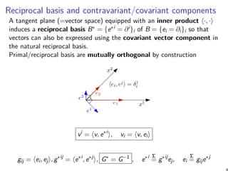
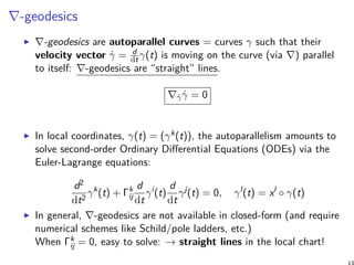
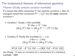
![Dual Pythagorean theorems
Any pair of points can either be linked using the ∇-geodesic (θ-straight
[PQ]) or the ∇∗-geodesic (η-straight [PQ]∗).
→ There are 23 = 8 geodesic triangles.
P
Q
R
P
Q
R
D(P : R) = D(P : Q) + D(Q : R)
BF (θ(P) : θ(R)) = BF (θ(P) : θ(Q)) + BF (θ(Q) : θ(R))
D∗
(P : R) = D∗
(P : Q) + D∗
(Q : R)
BF ∗ (η(P) : η(R)) = BF ∗ (η(P) : η(Q)) + BF ∗ (η(Q) : η(R))
γ∗
(P, Q) ⊥F γ(Q, R)
γ(P, Q) ⊥F γ∗
(Q, R)
γ∗
(P, Q) ⊥F γ(Q, R) ⇔ (η(P) − η(Q))⊤
θ(Q) − θ(R) = 0
γ(P, Q) ⊥F γ∗
(Q, R) ⇔ (θ(P) − θ(Q))⊤
η(Q) − η(R) = 0](https://image.slidesharecdn.com/introig-inriaoct2-2018-181004165425/85/An-elementary-introduction-to-information-geometry-26-320.jpg)
![Fisher Information Matrix (FIM), positive semi-definite
Parametric family of probability distributions P := {pθ(x)}θ for
θ ∈ Θ
Likelihood function L(θ; x) and log-likelihood function
l(θ; x) := log L(θ; x)
Score vector sθ = ∇θl = (∂il)i indicates the sensitivity of the
likelihood ∂il :=: ∂
∂θi
l(θ; x)
Fisher information matrix (FIM) of D × D for dim(Θ) = D:
PI(θ) := Eθ [∂il∂jl]ij ≽ 0
Cramér-Rao lower bound1 on the variance of any unbiased estimator
Vθ[ˆθn(X)] ≽
1
n
PI−1
(θ)
FIM invariant by reparameterization of the sample space X, and
covariant by reparameterization of the parameter space Θ.
1F. Nielsen. “Cramér-Rao lower bound and information geometry”. In: Connected at
Infinity II. Springer, 2013.](https://image.slidesharecdn.com/introig-inriaoct2-2018-181004165425/85/An-elementary-introduction-to-information-geometry-29-320.jpg)
![Some examples of Fisher information matrices
FIM of an exponential family: Include Gaussian, Beta, ∆D, etc.
E =
{
pθ(x) = exp
( D∑
i=1
ti(x)θi − F(θ) + k(x)
)
such that θ ∈ Θ
}
F is the strictly convex cumulant function
EI(θ) = Covθ[t(X)] = ∇2
F(θ) = ∇2
F∗
(η)−1
≻ 0
FIM of a mixture family: Include statistical mixtures, ∆D
M =
{
pθ(x) =
D∑
i=1
θiFi(x) + C(x) such that θ ∈ Θ
}
with {Fi(x)}i linearly independent on X,
∫
Fi(x)dµ(x) = 0 and∫
C(x)dµ(x) = 1
MI(θ) = Eθ
[
Fi(x)Fj(x)
p2
θ(x)
]
=
∫
X
Fi(x)Fj(x)
pθ(x)
dµ(x) ≻ 0](https://image.slidesharecdn.com/introig-inriaoct2-2018-181004165425/85/An-elementary-introduction-to-information-geometry-30-320.jpg)
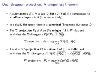
![Expected α-geometry from expected dual α-connections
Fisher “information metric” tensor from FIM (regular models)
Pg(u, v) := (u)⊤
θ PIθ(θ)(v)θ ≻ 0
Exponential connection and mixture connection:
P∇e
:= Eθ [(∂i∂jl)(∂kl)] , P∇m
:= Eθ [(∂i∂jl + ∂il∂jl)(∂kl)]
Dualistic structure (P, Pg, m
P ∇, e
P∇) with cubic skewness tensor:
Cijk = Eθ [∂il∂jl∂kl]
It follows a one-family of α-CCMs: {(P, Pg, P∇−α, P∇+α)}α with
PΓαk
ij := −
1 + α
2
Cijk = Eθ
[(
∂i∂jl +
1 − α
2
∂il∂jl
)
(∂kl)
]
P∇−α + P∇α
2
= LC
P ∇ := LC
∇(Pg)
In case of an exponential family E or a mixture family M, we get
Dually Flat Manifolds (Bregman geometry/ std f-divergence)
e
MΓ = m
MΓ = e
EΓ = m
E Γ = 0](https://image.slidesharecdn.com/introig-inriaoct2-2018-181004165425/85/An-elementary-introduction-to-information-geometry-31-320.jpg)
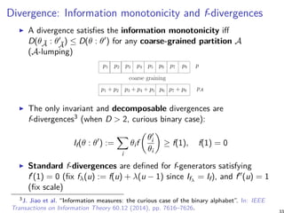
![Properties of Csiszár-Ali-Silvey f-divergences
Statistical f-divergences are invariant4 under one-to-one/sufficient
statistic transformations y = t(x) of the sample space:
p(x; θ) = q(y(x); θ).
If[p(x; θ) : p(x; θ′
)] =
∫
X
p(x; θ)f
(
p(x; θ′)
p(x; θ)
)
dµ(x)
=
∫
Y
q(y; θ)f
(
q(y; θ′)
q(y; θ)
)
dµ(y)
= If[q(y; θ) : q(y; θ′
)]
Dual f-divergences for reference duality:
If
∗
[p(x; θ) : p(x; θ′
)] = If[p(x; θ′
) : p(x; θ)] = If⋄ [p(x; θ) : p(x; θ′
)]
for the standard conjugate f-generator (diamond f⋄ generator):
f⋄
(u) := uf
(
1
u
)
4Y. Qiao and N. Minematsu. “A Study on Invariance of f-Divergence and Its Application to
Speech Recognition”. In: IEEE Transactions on Signal Processing 58.7 (2010), pp. 3884–3890.](https://image.slidesharecdn.com/introig-inriaoct2-2018-181004165425/85/An-elementary-introduction-to-information-geometry-34-320.jpg)
![Some common examples of f-divergences
The family of α-divergences:
Iα[p : q] :=
4
1 − α2
(
1 −
∫
p
1−α
2 (x)q1+α
(x)dµ(x)
)
obtained for f(u) = 4
1−α2 (1 − u
1+α
2 ), and include
Kullback-Leibler KL[p : q] =
∫
p(x) log p(x)
q(x) dµ(x) for f(u) = − log u
(α = 1)
reverse Kullback-Leibler KL∗
[p : q] =
∫
q(x) log q(x)
p(x) dµ(x) for
f(u) = u log u (α = −1)
squared Hellinger divergence H2
[p : q] =
∫
(
√
p(x) −
√
q(x))2
dµ(x)
for f(u) = (
√
u − 1)2
(α = 0)
Pearson and Neyman chi-squared divergences
Jensen-Shannon divergence (bounded):
1
2
∫ (
p(x) log
2p(x)
p(x) + q(x)
+ q(x) log
2q(x)
p(x) + q(x)
)
dµ(x)
for f(u) = −(u + 1) log 1+u
2 + u log u
Total Variation (metric) 1
2
∫
|p(x) − q(x)|dµ(x) for f(u) = 1
2|u − 1|](https://image.slidesharecdn.com/introig-inriaoct2-2018-181004165425/85/An-elementary-introduction-to-information-geometry-35-320.jpg)
![Invariant f-divergences yields Fisher metric/α-connections
Invariant (separable) standard f-divergences related infinitesimally to
the Fisher metric:
If[p(x; θ) : p(x; θ + dθ)] =
∫
p(x; θ)f
(
p(x; θ + dθ)
p(x; θ)
)
dµ(x)
Σ
=
1
2
Fgij(θ)dθi
dθj
A statistical parameter divergence on a parametric family of
distributions yield an equivalent parameter divergence:
PD(θ : θ′
) := DP[p(x; θ) : p(x; θ′
)]
Thus we can build the information-geometric structure induced by
this parameter divergence PD(· : ·)
For PD(· : ·) = If[· : ·], the induced ±1-divergence connections
If
P∇ := P If ∇ and
(If)∗
P ∇ := P I∗
f ∇ are the expected ±α-connections
with α = 2f′′′(1) + 3. +1/ − 1-connection =e/m-connection](https://image.slidesharecdn.com/introig-inriaoct2-2018-181004165425/85/An-elementary-introduction-to-information-geometry-36-320.jpg)
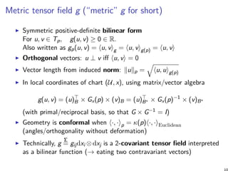
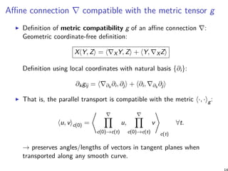
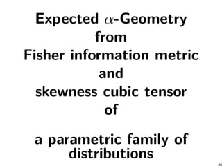
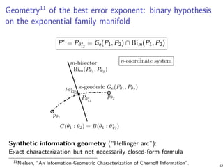
![Bayesian Hypothesis Testing/Binary classification7
Given two distributions P0 and P1, classify observations X1:n (= decision
problem) as either iid sampled from P0 or from P1? For example, P0 =
signal, P1 = noise (assume same prior w1 = w2 = 1
2)
x1 x2
p0(x) p1(x)
x
Assume P0 ∼ Pθ0
, P1 ∼ Pθ1
∈ E belong to an exponential family
manifold E = {Pθ} with dually flat structure (E, Eg, E∇e, E∇m).
This structure can also be derived from a divergence manifold
structure (E, KL∗
).
Therefore KL[Pθ : Pθ′ ] amounts to a Bregman divergence (for the
cumulant function of the exponential family):
KL[Pθ : Pθ′ ] = BF(θ′
: θ)](https://image.slidesharecdn.com/introig-inriaoct2-2018-181004165425/85/An-elementary-introduction-to-information-geometry-40-320.jpg)
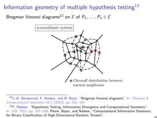
![Hypothesis Testing (HT)/Binary classification10
The best exponent error8 α∗ of the best Maximum A Priori (MAP)
decision rule is found by minimizing the Bhattacharyya distance to get
the Chernoff information:
C[P1, P2] = − log min
α∈(0,1)
∫
x∈X
pα
1 (x)p1−α
2 (x)dµ(x) ≥ 0,
On E, the Bhattacharyya distance amounts to a skew Jensen
parameter divergence9:
J
(α)
F (θ1 : θ2) = αF(θ1) + (1 − α)F(θ2) − F(θ1 + (1 − α)θ2),
Theorem: Chernoff information = Bregman divergence for exponential
families at the optimal exponent value:
C[Pθ1
: Pθ2
] = B(θ1 : θ
(α∗)
12 ) = B(θ2 : θ
(α∗)
12 )
8G.-T. Pham, R. Boyer, and F. Nielsen. “Computational Information Geometry for Binary
Classification of High-Dimensional Random Tensors”. In: Entropy 20.3 (2018), p. 203.
9F. Nielsen and S. Boltz. “The Burbea-Rao and Bhattacharyya centroids”. In: IEEE
Transactions on Information Theory 57.8 (2011).
10Nielsen, “An Information-Geometric Characterization of Chernoff Information”.](https://image.slidesharecdn.com/introig-inriaoct2-2018-181004165425/85/An-elementary-introduction-to-information-geometry-41-320.jpg)
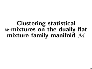
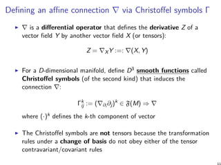
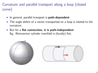
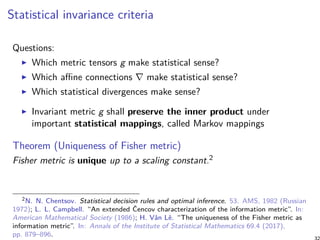
![Dually flat mixture family manifold14
Consider D + 1 prescribed component distributions {p0, . . . , pD} and
form the mixture manifold M by considering all their convex weighted
combinations M = {mθ(x) =
∑D
i=0 wipi(x)}
0
0.05
0.1
0.15
0.2
0.25
0.3
0.35
0.4
0.45
0.5
-4 -2 0 2 4 6 8
M1
M2
Gaussian(-2,1)
Cauchy(2,1)
Laplace(0,1)
Information-geometric structure: (M, Mg, M∇−1, M∇1) is dually flat
and equivalent to (Mθ, KL). That is, the KL between two mixtures with
prescribed components is equivalent to a Bregman divergence.
KL[mθ : mθ′ ] = BF(θ : θ′
), F(θ) = −h(mθ) =
∫
mθ(x) log mθ(x)dµ(x)
14F. Nielsen and R. Nock. “On the geometric of mixtures of prescribed distributions”. In:
IEEE ICASSP. 2018. 45](https://image.slidesharecdn.com/introig-inriaoct2-2018-181004165425/85/An-elementary-introduction-to-information-geometry-45-320.jpg)
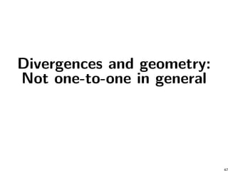

This document provides an elementary introduction to information geometry. It discusses how information geometry generalizes concepts from Riemannian geometry to study the geometry of decision making and model fitting. Specifically, it introduces: 1. Dually coupled connections (∇, ∇*) that are compatible with a metric tensor g and define dual parallel transport on a manifold. 2. The fundamental theorem of information geometry, which states that manifolds with dually coupled connections (∇, ∇*) have the same constant curvature. 3. Examples of statistical manifolds with dually flat geometry that arise from Bregman divergences and f-divergences, making them useful for modeling relationships between probability distributions


![谷歌留痕技术 [ 𝙩𝙤𝙥 𝟮𝟯𝟯. 𝙘 𝙤𝙢 ]](https://cdn.slidesharecdn.com/ss_thumbnails/top233-260130174328-3833018c-thumbnail.jpg?width=640&height=640&fit=bounds)


