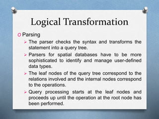
Algorithms for Query Processing and Optimization of Spatial Operations

Algorithms for Spatial Joins
and Spatial Query Processing
and Optimization
-Natasha Mandal

Applications of Spatial Queries
O Spatial Database Systems
O Geographical Information Systems
O Urban Planning
O CAD/CAM systems
O Image Databases

NEAREST
NEIGHBOR
QUERY
RANGE
QUERY
MAP
OVERLAY

Goals
O Understand more about Query Processing in
SDBMS
O Learn more about Spatial Operations in SDBMS
O Learn about Optimization in SDBMS

What is Query Processing?
Why Optimize?
O Queries are expressed in a high-level declarative
language such as SQL.
O The database software is supposed to map the
query into a sequence of operations supported by
spatial indexes and storage structures.
O Goals:
 Process a query accurately
 Do this in the minimum amount of time possible

What is Query Processing?
Why Optimize?
O Queries are composed of a basic set of relations.
O Query processing and optimization are divided into
two steps:
 Design and fine-tune algorithms for each of the
basic relational operators.
 Map high-level queries into a composition of these
basic relational operators and optimize (using
information in the first step).

Challenges in Spatial Databases
 Unlike relational databases, spatial databases
have no fixed set of operators that serve as
building blocks for query evaluation (ex. Overlap
and Intersect may return a similar result).
 Spatial databases have large volumes of complex
objects (with spatial extensions) which cannot be
sorted in a one-dimensional array.
 The assumption that I/O costs dominate CPU
costs is no longer valid since computationally
expensive algorithms are used to test for spatial
predicates.

Spatial Operations
O Spatial Operations can be classified into four
groups:
 Update - Modify, Create etc.
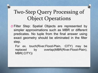
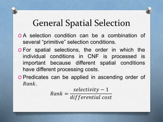
 Selection –
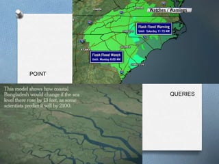
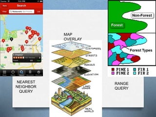
o Point Query (𝑃𝑄): Given a query point 𝑝, find all spatial
objects 𝑂 that contain it:
𝑃𝑄 𝑝 = {𝑂|𝑝 ∈ 𝑂. 𝐺 ≠ ∅}
where 𝑂. 𝐺 is the geometry of the object 𝑂.
Ex. “Find all river flood-plains which contain the CITY” [CITY
is assumed to be a point type]
o Range Query (𝑅𝑄): Given a query polygon 𝑃, find all spatial
objects 𝑂 which intersect 𝑃. [If 𝑃 is a rectangle, 𝑅𝑄 is a
window query]
𝑅𝑄(𝑃)={𝑂│𝑂.‫ܩ‬ ∧ 𝑃.‫}∅≠ܩ‬
Ex. “Get all forests which overlap with flood plain of River
Nile”

Spatial Operations
 Spatial Join – This relation holds when two
tables 𝑅 and 𝑆 are joined on a spatial predicate
𝜃 . Map Overlay is an important variant of
Spatial Join.
𝑅 ⋈ 𝜃 𝑆 = 𝑜1, 𝑜2 𝑜1 ∈ 𝑅, 𝑜2 ∈ 𝑆, 𝜃 𝑜1. 𝐺, 𝑜2. 𝐺
Some example 𝜃 predicates are intersect, contains,
is enclosed by, distance, northwest, adjacent,
meets, overlap etc.

Spatial Operations
Ex. “Find all forest stands and river plains which
overlap”
SELECT FS.name, FP.name
FROM Forest Stand FS, Flood Plain FP
WHERE overlap(FS.G, FP.G)
 Spatial Aggregate – These are usually variants of
the nearest neighbor search.
𝑁𝑁𝑄 𝑜′ = {𝑜|∀𝑜": 𝑑𝑖𝑠𝑡(𝑜′. 𝐺, 𝑜. 𝐺) ≤ 𝑑𝑖𝑠𝑡(𝑜′. 𝐺, 𝑜". 𝐺)}

Two-Step Query Processing of
Object Operations
O Filter Step: Spatial Objects are represented by
simpler approximations such as MBR or different
predicates. No tuple from the final answer using
exact geometry should be eliminated in the filter
step.
For ex. touch(River.Flood-Plain, :CITY) may be
replaced by overlap(MBR(River.Flood-Plain),
MBR(:CITY))

Two-Step Query Processing of
Object Operations
 Refinement Step: The exact geometry of each
element from the candidate set and the exact
predicate are examined. This may require a CPU
intensive application and may be processed
outside the spatial database (in a GIS).
Filtering – MBRs
Geometric Filter (Approximations) – Convex Hull,
Minimum Enclosed Circle etc.
Exact Geometry – Plane Sweep etc.

Techniques for Spatial Selection
O What are the alternative ways of processing a
query? It depends on how the file containing the
relations being queried is organized.
 Unsorted Data and No Index – Use brute force to
scan the whole file and test each record for the
predicate.
 Spatial Indexing – Can be used to access geometric
data. The MBRs of spatial attributes of a relation
can be indexed.
 Space filling curves – These can be used to map
points of multidimensional space into one
dimensional space. A B-Tree index can be imposed
on ordered entries to enhance the search.

General Spatial Selection
O A selection condition can be a combination of
several “primitive” selection conditions.
O For spatial selections, the order in which the
individual conditions in CNF is processed is
important because different spatial conditions
have different processing costs.
O Predicates can be applied in ascending order of
𝑅𝑎𝑛𝑘.
𝑅𝑎𝑛𝑘 =
𝑠𝑒𝑙𝑒𝑐𝑡𝑖𝑣𝑖𝑡𝑦 − 1
𝑑𝑖𝑓𝑓𝑒𝑟𝑒𝑛𝑡𝑖𝑎𝑙 𝑐𝑜𝑠𝑡

General Spatial Selection
𝑠𝑒𝑙𝑒𝑐𝑡𝑖𝑣𝑖𝑡𝑦 𝑝 =
𝑐𝑎𝑟𝑑𝑖𝑛𝑎𝑙𝑖𝑡𝑦(𝑜𝑢𝑡𝑝𝑢𝑡(𝑝))
𝑐𝑎𝑟𝑑𝑖𝑛𝑎𝑙𝑖𝑡𝑦(𝑖𝑛𝑝𝑢𝑡(𝑝))
𝑑𝑖𝑓𝑓𝑒𝑛𝑡𝑖𝑎𝑙 𝑐𝑜𝑠𝑡 = per tuple cost of a predicate. It
remains constant throughout the life of the function
and can be stored in the system catalog (along with
selectivity).

Spatial Join
O Spatial Join can be an expensive operation and
the presence of indices can help in the fast
processing of queries.
Classification of spatial join methods
Both inputs are indexed One input is indexed Neither input is indexed
 transformation to z-values
 spatial join index
 tree matching
 index nested loops
 seeded tree join
 build and match
 sort and match
 slot index spatial join
 spatial hash join
 partition based spatial merge join
 size separation spatial join
 scalable sweeping-based spatial join

The R-Tree Join
O This algorithm can be used when both the inputs
are indexed.
O It is based on the enclosure property of trees: if
two nodes do not intersect, then there are no
rectangles below them that can intersect.
O RJ starts from the roots of the trees to be joined
and finds pairs of overlapping entries.
O For each such pair, the algorithm is recursively
called until the leaf levels where overlapping pairs
constitute solutions.
O The following algorithm assumes both the R-Trees
are of equal height (this can easily be extended).

The R-Tree Join
Alg. RJ(Rtree_Node ni, RTNode nj)
for each entry ej,y ∈ nj, do
{
for each entry ei,x ∈ ni with ei,x ⋂, ej,y ≠ ∅ do
{
if ni is a leaf node /* nj is also a leaf node */
then Output (ei,x, ej,y );
else /* intermediate nodes */
{
ReadPage(ei,x. ref); ReadPage(ej,y.ref);
RJ(ei,x ref, ej,y ref);
}
}
} /* end for */

The R-Tree Join
 Optimizations for CPU speed:
 Search Space Restriction
 Plane Sweep – sorting in one dimension
reduces time for finding overlapping pairs
 Optimizations for I/O speed:
 Plane Sweep - consecutive computed
pairs overlap with high probability
 Breadth-first traversal that sorts the output
at each level in order to reduce the
number of page accesses.

Spatial Hash Join
O This algorithm can be used to compute
the join of two non-indexed datasets 𝑅
(build input i.e. smaller relation) and 𝑆
(probe input).
O 𝑅 is partitioned into 𝐾 buckets.
 The initial buckets are points determined
based on sampling.
 Each object is inserted into the bucket that
is enlarged the least.

Spatial Hash Join
O 𝑆 is hashed into buckets with the same extent
as 𝑅's buckets
 An object is inserted into all buckets that intersect
it.
 Some objects may be assigned to multiple buckets
(replication) and some may not be inserted at all
(filtering).
O The two bucket sets are joined; each bucket from
R is matched with only one bucket from S, thus
requiring a single scan of both files.
O If for some pair neither bucket fits in memory, an
R-tree is built for one of them, and the bucket-to-
bucket join is executed in an index nested loop
fashion.

Slot Index Spatial Join
O This algorithm is applicable when there is an
R-tree for one of the inputs (𝑅).
O If 𝐾 is the desired number of partitions, SISJ
will find the topmost level of the tree such that
the number of entries is larger than or equal
to 𝐾. These entries are then grouped into 𝐾
(possibly overlapping) partitions called slots.
 Each slot contains the MBR of the indexed R-
tree entries, along with a list of pointers to
these entries.

 SISJ starts with a single empty slot and inserts
entries into the slot that is enlarged the least.
 When the maximum capacity of a slot is reached
(determined by 𝐾 and the total number of entries),
either some entries are deleted and reinserted or
the slot is split according to the R*-tree splitting
policy.
O The second dataset 𝑆 is hashed into buckets with
the same extents as the slots.
 If an object from 𝑆 does not intersect any bucket, it
is filtered.
 If it intersects more than one bucket, it is replicated.

O The join phase
 All data from the R-tree of 𝑅 indexed by a slot
are loaded and joined with the corresponding
hash-bucket from 𝑆 using plane sweep.
 If the data to be joined does not fit in memory,
they can be joined using an algorithm which
employs external sorting and then plane
sweep.
 During the join phase of SISJ, when no data
from 𝑆 is inserted into a bucket, the sub-tree
data under the corresponding slot is not
loaded (slot filtering).

Query Optimization
O The metric used for an evaluation plan is time
required to execute the query. For spatial
databases this would include I/O and CPU costs.
O A query optimizer (a module in the database
software) generates different evaluation plans and
determines the appropriate execution strategy.
O The idea is to avoid the worst plans and choose a
good one (seldom the best one).
O The procedures of query optimizer can be divided
into two parts - 𝑙𝑜𝑔𝑖𝑐𝑎𝑙 𝑡𝑟𝑎𝑛𝑠𝑓𝑜𝑟𝑚𝑎𝑡𝑖𝑜𝑛 and
𝑑𝑦𝑛𝑎𝑚𝑖𝑐 𝑝𝑟𝑜𝑔𝑟𝑎𝑚𝑚𝑖𝑛𝑔.

Logical Transformation
O Parsing
 The parser checks the syntax and transforms the
statement into a query tree.
 Parsers for spatial databases have to be more
sophisticated to identify and manage user-defined
data types.
 The leaf nodes of the query tree correspond to the
relations involved and the internal nodes correspond
to the operations.
 Query processing starts at the leaf nodes and
proceeds up until the operation at the root node has
been performed.

SELECT L.Name FROM
Lake L, Facilities Fa
WHERE Area(L.G)>20
AND Fa.Name
=“Campground” AND
Distance(Fa.G, L.G)<50
𝜋 𝐿.𝑁𝑎𝑚𝑒
𝜎𝐴𝑟𝑒𝑎.𝐺>20
𝜎 𝐹𝑎.𝑁𝑎𝑚𝑒="𝐶𝑎𝑚𝑝𝑔𝑟𝑜𝑢𝑛𝑑"
⋈ 𝐷𝑖𝑠𝑡𝑎𝑛𝑐𝑒 𝐹𝑎.𝐺,𝐿.𝐺 <50
𝐿𝑎𝑘𝑒 𝐿 𝐹𝑎𝑐𝑖𝑙𝑖𝑡𝑖𝑒𝑠 𝐹𝑎

O Logical Transformation
 The query tree generated by parser is mapped onto
equivalent query trees (based on a formal set of
rules inherited from relational algebra).
 After equivalent trees are enumerated, we can apply
heuristics to filter out non-candidates.
 Clear-cut heuristic may not apply for spatial
databases due to user-defined functions etc.
 𝑅𝑎𝑛𝑘 can be used as a heuristic. 𝑆𝑒𝑙𝑒𝑐𝑡𝑖𝑣𝑖𝑡𝑦 and
𝑑𝑖𝑓𝑓𝑒𝑟𝑒𝑛𝑡𝑖𝑎𝑙 𝑐𝑜𝑠𝑡 can be stored in the System
Catalog.

O Equivalence Rules:
 Selections
o 𝜎𝑐1∧𝑐2∧⋯𝑐𝑛(𝑅) ≡ 𝜎𝑐1(𝜎𝑐2 … 𝜎𝑐𝑛 𝑅 … ) – Can push all
non-spatial conditions towards the right.
o 𝜎𝑐1(𝜎𝑐2 𝑅 ) ≡ 𝜎𝑐2(𝜎𝑐1 𝑅 )
 Projections
o 𝜋 𝑎1(𝑅) ≡ 𝜋 𝑎1 𝜋 𝑎2 … 𝜋 𝑎𝑛 𝑅 … if 𝑎𝑖 ⊂ 𝑎𝑖+1for 𝑖 =
1, … 𝑛 − 1
 Cross Product and Joins
o 𝑅 ⋈ 𝑆 ≡ 𝑆 ⋈ 𝑅
o 𝑅 ⋈ (𝑆 ⋈ 𝑇) ≡ (𝑅 ⋈ 𝑆) ⋈ 𝑇

 Selection, Projection and Joins
o If the selection condition involves attributes retained by
the projection operator
𝜋 𝑎(𝜎𝑐 𝑅 ) ≡ 𝜎𝑐(𝜋 𝑎 𝑅 )
o If a selection condition involves only an attribute that is
present in 𝑅 and not in 𝑆 then
𝜎𝑐(𝑅 ⋈ 𝑆) ≡ 𝜎𝑐(𝑅) ⋈ 𝑆
o Projection can be computed with a join:
𝜋 𝑎(𝑅 ⋈ 𝑆) ≡ 𝜋 𝑎1(𝑅) ⋈ 𝜋 𝑎2(𝑆)
where 𝑎1 ⊆ 𝑎 which appears in 𝑅 and 𝑎2 ⊆ 𝑎 which
appears in 𝑆

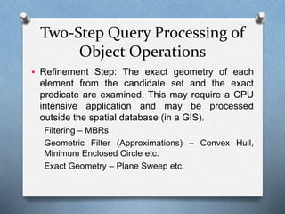
Cost Based Optimization:
Dynamic Programming
O Dynamic Programming is used to determine the
optimal execution strategy from a set of execution
plans.
O The optimal solution minimizes the cost function.
O We focus on each node of query tree and enumerate
the different execution strategies available to process
the node. The different processing strategies for each
node when combined for the whole query constitutes
the plan space.
O The cardinality of plan space might be high and the
optimization time must be kept minimum. This
suggests that we should select a good (not the best)
plan.

Dynamic Programming
O The factors that a good cost function must take
into account are:
o Access cost – Searching for and transferring data
from secondary storage.
o Storage cost – Storing intermediate temporary
relations produced by an execution strategy.
o Computation cost – CPU cost of performing in-
memory operations.
o Communication cost – Transferring information
between the client and server.

Dynamic Programming
O Systems Catalog
 It contains the information required by the cost
function to design an optimal execution strategy.
 It includes:
o the size of each file
o the number of records in each file
o number of blocks over which records are spread
o information about indexes and indexing attributes
o 𝑠𝑒𝑙𝑒𝑐𝑡𝑖𝑣𝑖𝑡𝑦 and 𝑑𝑖𝑓𝑓𝑒𝑟𝑒𝑛𝑡𝑖𝑎𝑙 𝑐𝑜𝑠𝑡
o can materialize expensive, user-defined functions
and index their values for fast retrieval

Dynamic Programming
O Cost Functions
𝑐𝑜𝑠𝑡 = 𝐸𝑥𝑝 𝑟𝑒𝑐𝑜𝑟𝑑𝑠_𝑒𝑥𝑎𝑚𝑖𝑛𝑒𝑑 + 𝐾 ∗ 𝐸𝑥𝑝(𝑝𝑎𝑔𝑒𝑠_𝑟𝑒𝑎𝑑)
 𝐸𝑥𝑝 𝑟𝑒𝑐𝑜𝑟𝑑𝑠_𝑒𝑥𝑎𝑚𝑖𝑛𝑒𝑑 = expected number of records read
[measure of CPU time]
 𝐸𝑥𝑝(𝑝𝑎𝑔𝑒𝑠_𝑟𝑒𝑎𝑑)= expected number of pages read from
storage [measure of I/O time]
 𝐾= measure of how important CPU resources are relative to
I/O resources
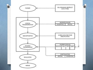
O Decomposition and Merge in Hybrid Architecture
 A query is decomposed into spatial and non-spatial part.
 Subqueries are optimized in separate modules and are
merged.

Conclusion
O We learnt about the 2-Step Query Processing
paradigm.
O We reviewed algorithms for Spatial Operations like
Spatial Join.
O We learnt how Dynamic Programming can be
used to optimize queries based on the cost
function.

Algorithms for Query Processing and Optimization of Spatial Operations

Algorithms for Query Processing and Optimization of Spatial Operations

More Related Content

What's hot

Similar to Algorithms for Query Processing and Optimization of Spatial Operations

Recently uploaded

Algorithms for Query Processing and Optimization of Spatial Operations