This document discusses algorithmic research problems and different types of algorithms used to solve them. It begins by defining an algorithm and providing examples of common algorithm types like search, sorting, shortest path, and more. It then covers different types of algorithmic problems like polynomial problems, which can be solved in polynomial time by polynomial algorithms, and NP-hard or combinatorial problems, which typically require exponential algorithms. Several examples are given of problems that fall into each category. The document also discusses how problem complexity is analyzed and how it relates to the algorithm types.

2. Introduction
Algorithmic Research
Problems
Types of Algorithmic
research problems

3. Algorithm:
It is a sequence steps to solve
a problem of interest.
It is procedure for solving
problem with special focus on
solving
problem
using
computer.

4. Search algorithms
Sorting algorithms
Shortest path algorithms
Minimum spanning tree algorithms
Branch and bound algorithms
Hungerian method for assignment
method

5. Simplex algorithm for linear
programming
Zero-one implicit enumeration
algorithm for 0-1 programming
Simulated annealing algorithm
Genetic algorithm
Tabu search algorithm
Greedy algorithm for Travelling
Salesman Problem

6. Introduction
Algorithmic Research
Problems
Types of Algorithmic
research problems

7. Financial
management
Marketing
management
Production
management
Research
problems in
different
functional areas
of management
Personnel
management
Other areas

8. Minimizing the mean tardiness in
single scheduling problem
Minimizing the weighted mean
tardiness
in
single
machine
scheduling problem
Minimizing the sum of the tardiness
and earliness in single machine
scheduling problem
Minimizing the makespan in parallel
machines scheduling problem

9. Minimizing the makespan in flowshop
scheduling problem
Maximizing the balancing efficiency of
an assembly line
Resource leveling and allocation in
project network
Aggregate planning problem
Master production planning problem

10. Dealer
location
problem
Travelling
Salesman problem
Problems in
Marketing
Management
Media
planning
problem
Salesman
assignment
problem

11. Determination of
rate of return
Capital budgeting
Exclusive
Selection of
mutually and
collectively
exhaustive
projects
Portfolio
management

12. Problems in Personnel
Management
Allocation
Employees
in-house
training
problem
Manpower
planning
problem
of fund to
personnel
activities
Assignmen
for
t problem
improved
labor
productivit
y

13. Fire
station
s
locatio
n
proble
m
Schools
locatio
n
proble
m
Branch
banks
locatio
n
proble
m
Schedu
ling
process
ors in
parallel
comput
ers
Encrypt
ion and
decrypt
ion
Organiz
ation of
B-tree.

14. Introduction
Algorithmic Research
Problems
Types of algorithmic
Research Problems

15. Algorithmic
problems
Polynomial
problem
Combinational/
NP-hard
problems
The algorithms for
solving these real
life problems
Polynomial
algorithms
Exponential
algorithms

16. If the complexity of an algorithm for a
problem is in polynomial form, then that
algorithm is known as polynomial algorithm.
It will take finite times to solve a problem
optimally.
The complexity of an algorithm means a
function representing the number of steps
required to solve a problem under the worst
case behavior.
An algorithm consists of a set of steps.
For some problems, the algorithm will be
executed for all its steps or for its subset of

17. The complexity of an algorithm,
n – problem size
f(n) – the time complexity function
The function is a polynomial order 4.
The algorithm which has this function as its
complexity function is known as polynomial
function
The worst case behavior of the algorithm is
known as order of the algorithm.
The highest polynomial of the given
function is treated to be worst case.

18. The problems which will have polynomial time
complexity function are called polynomial problems.
These problems are solved in finite time
Examples of polynomial problem
Shortest path problem
Finding the roots of a quadratic equation
Minimizing mean flow time in single machine
scheduling – SPT rule(Shortest Path Time)
Minimizing the maximum tardiness in single
machine scheduling problem – EDD(Earliest due
date) rule is used
Minimizing the make span in 2 machines and n
jobs case flow shop scheduling problem –
Johnson’s algorithm is used for this problem.

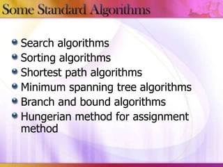
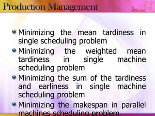
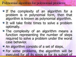
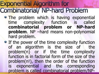
19. Step 1: Set k=0
Step 2: From the initial distance matrix [D⁰]
and the initial precedence matrix[P⁰] from
the distance network
Step 3: Set k = k+1
Step 4: Obtain the values of the distance
matrix, [ ] for all the cells, where i is not
equal to j using the following formula:
Step 5: Obtain the values of the precedence

20. Step 6: if k=n go to step 7, otherwise, set
k=k+1 and go to step-4
Step 7:Trace the shortest path for a given
combination of source node and destination
node
7.1 : X-Source node, Y-Destination node
7.2 : Fix Y node as the last node in the partially
formed shortest path
7.3: find the value from the final precedence
matrix for the row corresponding to node X
and the column corresponding to Y. Let it be Q.
Prefix node Q in the partially formed shortest
path.

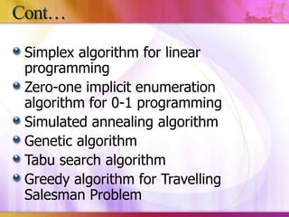
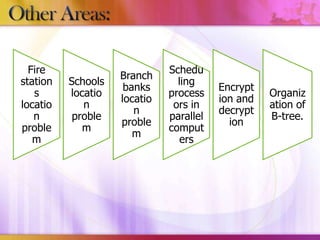
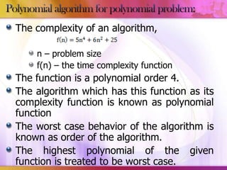
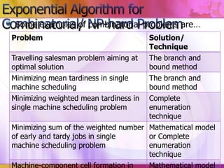
21. Critical analysis of execution of steps are
presented
The step-1 is executed only once.
The step-2 will be executed n² times to read
the distance matrix, [Dº]as well as the
precedence matrix[Pº]
Step-3 is repeated for one more time
In each of the step-4 and the step-5,
calculations for n² cells in the distance matrix,
as well as in the precedence matrix,
are
done for n times.
The step-6 is repeated for n times.

22. Based on the explanations from (a) to (f),
the time complexity function of Floyd’s
algorithm is,
f(n) =
= 1+ 2a₂nᶟ+(1+a₃)n
a₁, a₂ , a₃ - Constants
The highest degree of the above polynomial
is 3
The worst case complexity function of
Floyd’s algorithm is O(nᶟ
)
Floyd’s algorithm is a polynomial algorithm.
This algorithm gives the optimal solution in

23. 1
D0 =
5
2
0
4
2
0
-3
0
2
3
3
1
2
5
1
3
4
3
2
W=
1
2
-3
1
P=
0
0
0
2
0
0
0
3
0
0
0

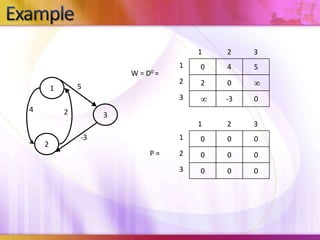
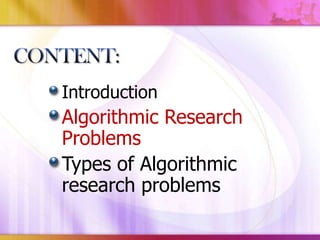
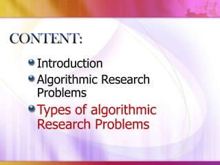
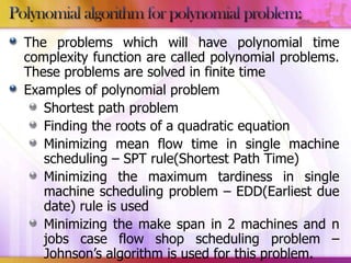
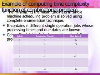
24. 1
4
2
1
D1 =
D0 =
5
2
-3
2
3
5
1
0
4
2
3
2
0
3
2
3
1
0
4
5
2
2
0
7
-3
-3
0
D1[2,3] = min( D0[2,3], D0[2,1]+D0[1,3] )
= min ( , 7)
=7
0
3
1
2
3
1
P=
1
0
0
0
2
0
0
1
3
0
0
0
D1[3,2] = min( D0[3,2], D0[3,1]+D0[1,2] )
= min (-3, )
= -3

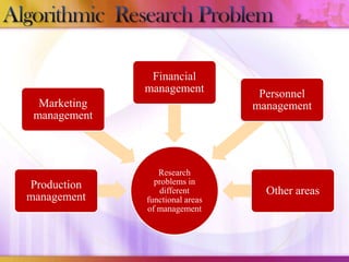
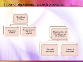
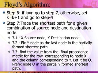
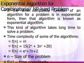
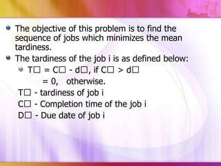
25. 1
1
4
2
D1 =
5
2
-3
0
4
5
2
2
0
7
-3
0
3
2
3
1
0
4
5
2
2
0
7
3
-1
-3
2
D2[1,3] = min( D1[1,3], D1[1,2]+D1[2,3] )
= min (5, 4+7)
=5
0
1
3
1
P=
3
1
3
1
D2 =
2
0
0
0
2
0
0
1
3
2
0
0
D2[3,1] = min( D1[3,1], D1[3,2]+D1[2,1] )
= min ( , -3+2)
= -1

26. If the time complexity function of an
algorithm for a problem is in exponential
form, then that algorithm is known as
exponential algorithm.
This kind of algorithm takes long time to
solve a problem.
Time complexity of some of the algorithms:
f(n) = n!
f(n) = 15(2ⁿ + 3n² +20)
f(n) = eⁿ+7n+2
n – Size of the problem

27. If a graphical plot is made for each of
these functions, the value of f(n) grows
exponentially.
This means that even for a small
increment in n will cause a very large
unproportionate positive in crease in
f(n).
The algorithm which are having such
functions are known as ‘exponential
algorithms’.
The order of complexity of the three
functions are O(n!), O(2ⁿ) and O(eⁿ)

28. The problem which is having exponential
time
complexity
function
is
called
combinatorial problem or NP-hard
problem. NP –hard means non-polynomial
hard problem.
If the power of the time complexity function
of an algorithm is the size of
the
problem(n) or if the time complexity
function is in factorial form of the size of the
problem(n!), then the order of the function
is exponential and the corresponding
problem is called combinatorial problem/NP-

29. Some examples of combinatorial problems are…
Problem
Travelling salesman problem aiming at
optimal solution
Minimizing mean tardiness in single
machine scheduling
Minimizing weighted mean tardiness in
single machine scheduling problem
Solution/
Technique
The branch and
bound method
The branch and
bound method
Complete
enumeration
technique
Minimizing sum of the weighted number Mathematical model
of early and tardy jobs in single
or Complete
machine scheduling problem
enumeration
technique
Machine-component cell formation in
Mathematical model

30. The minimizing the mean tardiness in single
machine scheduling problem is solved using
complete enumeration technique.
It contains n different single operation jobs whose
processing times and due dates are known.
Generalized data Processing Time(t)
of single machine scheduling
Job(i)
Due date(d)
problem
t₁
d₁
1
2
t₂
d₂
.
.
.
.
.
.
.
.
.
i
tᵢ
dᵢ
.
.
.
.
.
.
.
.
.
n
tn
dn

31. The objective of this problem is to find the
sequence of jobs which minimizes the mean
tardiness.
The tardiness of the job i is as defined below:
Tᶟ = Cᶟ - dᶟ, if Cᶟ > dᶟ
= 0, otherwise.
Tᶟ - tardiness of job i
Cᶟ - Completion time of the job i
Dᶟ - Due date of job i

32. Growth of no.of Sequences versus Problem
Size(n)
Problem Size (n) No.Of.Sequences(n
!)
1
2
1
2
3
6
4
5
6
7
8
9
10
24
120
720
5040
40320
362880
3628800