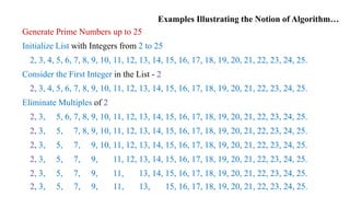
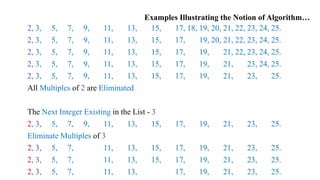
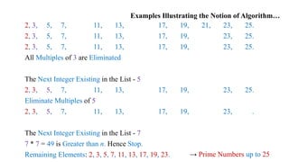
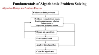
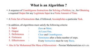
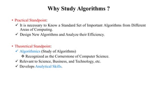
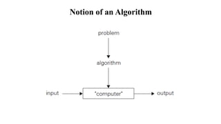
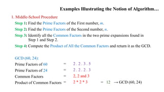
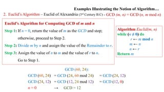
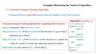
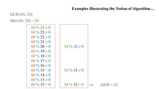
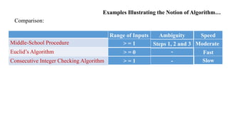
The document provides an introduction to algorithms, defining them as a sequence of instructions for solving problems with key criteria such as input, output, and definiteness. It emphasizes the necessity of studying algorithms for both practical and theoretical reasons, highlighting their significance in computer science. Various examples, such as the calculation of the greatest common divisor and the Sieve of Eratosthenes, illustrate different types of algorithms and the fundamentals of algorithm design and analysis.


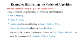
![Sieve of Eratosthenes
• Invented in Ancient Greece (200 B.C)
• Generates Consecutive Prime Numbers not exceeding Integer n > 1.
Sieve of Eratosthenes for Generating Prime Numbers up to n
Step 1: Initialize a list of Prime Candidates with consecutive
integers from 2 to n.
Step 2: Eliminate all Multiples of 2.
Step 3: Eliminate all Multiples of the Next Integer Remaining in
the list.
Step 4: Continue in this fashion until no more numbers can be
Eliminated.
Step 5: The Remaining Integers are the Primes needed.
Algorithm Seive (n)
For (p ← 2 to n) do A[p] ← p
For (p ←2 to 𝑛 ) do
If (A[p] ≠ 0)
j ← p ∗ p
While ( j ≤ n) do
A[j ] ← 0
j ← j + p
i ← 0
For (p ← 2 to n) do
If (A[p] ≠ 0)
L[i] ← A[p]
i ← i + 1
Return L
Note:
If p is a number whose multiples are being eliminated, then the First
Multiple existing is p * p because all smaller multiples. 2p, . . , (p − 1) p
have been eliminated on earlier passes through the list.
→ p * p Not Greater than n → p < 𝑛](https://image.slidesharecdn.com/01introductiontoalgorithms-240806082214-6c5a1122/85/Introduction-to-Algorithm-Design-and-Analysis-pdf-11-320.jpg)