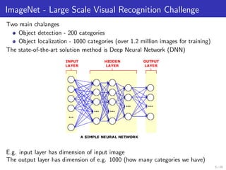
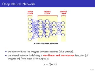
The document presents methods for solving large-scale machine learning problems, particularly using deep neural networks (DNN) in a distributed computing environment. It discusses various machine learning tasks, the structure of DNNs, and the challenges faced in distributed stochastic gradient descent algorithms, emphasizing the importance of mini-batch processing and model/data parallelism. It also touches upon advanced techniques like using Hessian information to improve convergence rates in optimization.

1. Solving Large-Scale Machine Learning Problems
in a Distributed Way
Martin Tak´aˇc
Cognitive Systems Institute Group Speaker Series
June 09 2016
1 / 28

2. Outline
1 Machine Learning - Examples and Algorithm
2 Distributed Computing
3 Learning Large-Scale Deep Neural Network (DNN)
2 / 28

3. Examples of Machine Learning
binary classification
classifies person to have cancer or not
decided for an input image to which class it belongs, e.g. car/person
spam detection/credit card fraud detection
multi-class classification
hand-written digits classification
speech understanding
face detection
product recommendation (collaborative filtering)
stock trading
. . . and many many others. . .
3 / 28

4. Support Vector Machines (SVM)
blue: healthy person
green: e.g. patient with lung cancer
Exhaled breath analysis for lung cancer: predict if patient has cancer or not
4 / 28

5. ImageNet - Large Scale Visual Recognition Challenge
Two main chalanges
Object detection - 200 categories
Object localization - 1000 categories (over 1.2 million images for training)
5 / 28

6. ImageNet - Large Scale Visual Recognition Challenge
Two main chalanges
Object detection - 200 categories
Object localization - 1000 categories (over 1.2 million images for training)
The state-of-the-art solution method is Deep Neural Network (DNN)
E.g. input layer has dimension of input image
The output layer has dimension of e.g. 1000 (how many categories we have)
5 / 28

7. Deep Neural Network
we have to learn the weights between neurons (blue arrows)
the neural network is defining a non-linear and non-convex function (of
weights w) from input x to output y:
y = f (w; x)
6 / 28

8. Example - MNIST handwritten digits recognition
A good w could give us
f







w;







=







0
0
0
0.991
...







f








w;








=







0
0
...
0
0.999







7 / 28

9. Mathematical Formulation
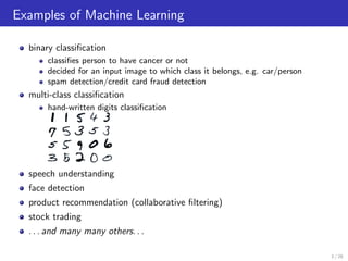
Expected Loss Minimization
let (X, Y ) be the distribution of input samples and its labels
we would like to find w such that
w∗
= arg min
w
E(x,y)∼(X,Y )[ (f (w; x), y)]
is a loss function, i.e. (f (w; x), y) = f (w; x) − y 2
8 / 28

10. Mathematical Formulation
Expected Loss Minimization
let (X, Y ) be the distribution of input samples and its labels
we would like to find w such that
w∗
= arg min
w
E(x,y)∼(X,Y )[ (f (w; x), y)]
is a loss function, i.e. (f (w; x), y) = f (w; x) − y 2
Impossible, as we do not know the distribution (X, Y )
8 / 28

11. Mathematical Formulation
Expected Loss Minimization
let (X, Y ) be the distribution of input samples and its labels
we would like to find w such that
w∗
= arg min
w
E(x,y)∼(X,Y )[ (f (w; x), y)]
is a loss function, i.e. (f (w; x), y) = f (w; x) − y 2
Impossible, as we do not know the distribution (X, Y )
Common approach: Empirical loss minimization:
we sample n points from (X, Y ): {(xi , yi )}n
i=1
we minimize regularized empirical loss
w∗
= arg min
w
1
n
n
i=1
(f (w; xi ), yi ) +
λ
2
w 2
8 / 28

12. Stochastic Gradient Descent (SGD) Algorithm
How can we solve
min
w
F(w) :=
1
n
n
i=1
(f (w; xi ); yi ) +
λ
2
w 2
9 / 28

13. Stochastic Gradient Descent (SGD) Algorithm
How can we solve
min
w
F(w) :=
1
n
n
i=1
(f (w; xi ); yi ) +
λ
2
w 2
1 we can use an iterative algorithm
2 we start with some initial w
3 we compute g = F(w)
4 we get a new iterate w ← w − αg
5 if w is still not good enough go to step 3
if n is very large, computing g can take a while.... even few hours/days
9 / 28

14. Stochastic Gradient Descent (SGD) Algorithm
How can we solve
min
w
F(w) :=
1
n
n
i=1
(f (w; xi ); yi ) +
λ
2
w 2
1 we can use an iterative algorithm
2 we start with some initial w
3 we compute g = F(w)
4 we get a new iterate w ← w − αg
5 if w is still not good enough go to step 3
if n is very large, computing g can take a while.... even few hours/days
Trick:
choose i ∈ {1, . . . , n} randomly
define gi = (f (w; wi ); yi ) + λ
2 w 2
use gi instead of g in the algorithm (step 4)
9 / 28

15. Stochastic Gradient Descent (SGD) Algorithm
How can we solve
min
w
F(w) :=
1
n
n
i=1
(f (w; xi ); yi ) +
λ
2
w 2
1 we can use an iterative algorithm
2 we start with some initial w
3 we compute g = F(w)
4 we get a new iterate w ← w − αg
5 if w is still not good enough go to step 3
if n is very large, computing g can take a while.... even few hours/days
Trick:
choose i ∈ {1, . . . , n} randomly
define gi = (f (w; wi ); yi ) + λ
2 w 2
use gi instead of g in the algorithm (step 4)
Note: E[gi ] = g, so in expectation, the ”direction” the algorithm is going is the
same as if we use the true gradient, but we can compute it n times faster!
9 / 28

16. Outline
1 Machine Learning - Examples and Algorithm
2 Distributed Computing
3 Learning Large-Scale Deep Neural Network (DNN)
10 / 28

17. The Architecture
What if the size of data {(xi , yi )} exceeds the memory of a single
computing node?
11 / 28

18. The Architecture
What if the size of data {(xi , yi )} exceeds the memory of a single
computing node?
each node can store portion of the data {(xi , yi )}
each node is connected to the computer network
they can communicate with any other node (over maybe 1 or more switches)
Fact: every communication is much more expensive then accessing local data
(can be even 100,000 times slower).
11 / 28

19. Outline
1 Machine Learning - Examples and Algorithm
2 Distributed Computing
3 Learning Large-Scale Deep Neural Network (DNN)
12 / 28

20. Using SGD for DNN in Distributed Way
assume that the size of data or the size weights (or both) is so big, that we
cannot store them on one machine
. . . or we can store them but it takes too long to compute something . . .
SGD: we need to compute w (f (w; xi ); yi )
The DNN has a nice structure
w (f (w; xi ); yi ) can we computed by backpropagation procedure (this is
nothing else just automated differentiation)
13 / 28

21. Why is SGD a Bad Distributed Algorithm
it samples only 1 sample and computes gi (this is very fast)
then w is updated
each update of w requires a communication (cost c seconds)
hence one iteration is suddenly much slower then if we would run SGD on
one computer
14 / 28

22. Why is SGD a Bad Distributed Algorithm
it samples only 1 sample and computes gi (this is very fast)
then w is updated
each update of w requires a communication (cost c seconds)
hence one iteration is suddenly much slower then if we would run SGD on
one computer
The trick: Mini-batch SGD
In each iteration
1 Choose randomly S ⊂ {1, 2, . . . , n} with |S| = b
2 Use gb = 1
b i∈S gi instead of just gi
14 / 28

23. Why is SGD a Bad Distributed Algorithm
it samples only 1 sample and computes gi (this is very fast)
then w is updated
each update of w requires a communication (cost c seconds)
hence one iteration is suddenly much slower then if we would run SGD on
one computer
The trick: Mini-batch SGD
In each iteration
1 Choose randomly S ⊂ {1, 2, . . . , n} with |S| = b
2 Use gb = 1
b i∈S gi instead of just gi
Cost of one epoch
number of MPI calls / epoch n/b
amount of data send over network n
b × log(N) × sizeof (w)
if we increase b → n we would minimize amount of data and number of
number of communications per epoch!
14 / 28

24. Why is SGD a Bad Distributed Algorithm
it samples only 1 sample and computes gi (this is very fast)
then w is updated
each update of w requires a communication (cost c seconds)
hence one iteration is suddenly much slower then if we would run SGD on
one computer
The trick: Mini-batch SGD
In each iteration
1 Choose randomly S ⊂ {1, 2, . . . , n} with |S| = b
2 Use gb = 1
b i∈S gi instead of just gi
Cost of one epoch
number of MPI calls / epoch n/b
amount of data send over network n
b × log(N) × sizeof (w)
if we increase b → n we would minimize amount of data and number of
number of communications per epoch! Caveat: there is no free lunch!
Very large b means slower convergence!
14 / 28

25. Model Parallelism
Model parallelism: we partition weights w across many nodes; every node
has all data points (but maybe just few features of them)
Hidden Layer 1
Hidden Layer 2
Output
Input
ForwardPropagation
Hidden Layer 1
Hidden Layer 2
Output
BackwardPropagation
Node1
Node1
Node2
Node2
AllSamples
AllSamples
AllSamples
AllSamples
Exchange Activation
Exchange Activation
Exchange Deltas
Exchange Deltas
15 / 28

26. Data Parallelism
Data parallelism: we partition data-samples across many nodes, each node
has a fresh copy of w
Hidden Layer 1
Hidden Layer 2
Output
Input
ForwardPropagation
Hidden Layer 1
Hidden Layer 2
Output
BackwardPropagation
Node1
Node1
Node2
Node2
PartialSamples
PartialSamples
PartialSamples
PartialSamples
Hidden Layer 1
Hidden Layer 2
Hidden Layer 1
Hidden Layer 2
Exchange Gradient
16 / 28

27. Large-Scale Deep Neural Network1
1Dipankar Das, Sasikanth Avancha, Dheevatsa Mudigere, Karthikeyan Vaidynathan, Srinivas
Sridharan, Dhiraj Kalamkar, Bharat Kaul, Pradeep Dubey: Distributed Deep Learning Using
Synchronous Stochastic Gradient Descent, arXiv:1602.06709
17 / 28

28. There is almost no speedup for large b
18 / 28

29. The Dilemma
large b allows algorithm to be efficiently run on large computer cluster (more
nodes)
very large b doesn’t reduce number of iterations, but each iteration is more
expensive!
The Trick: Do not use just gradient, but use also Hessian (Martens 2010)
19 / 28

30. The Dilemma
large b allows algorithm to be efficiently run on large computer cluster (more
nodes)
very large b doesn’t reduce number of iterations, but each iteration is more
expensive!
The Trick: Do not use just gradient, but use also Hessian (Martens 2010)
Caveat: Hessian matrix can be very large, e.g. the dimension of weights for
TIMIT datasets is almost 1.5M, hence to store Hessian we would need almost
10TB.
19 / 28

31. The Dilemma
large b allows algorithm to be efficiently run on large computer cluster (more
nodes)
very large b doesn’t reduce number of iterations, but each iteration is more
expensive!
The Trick: Do not use just gradient, but use also Hessian (Martens 2010)
Caveat: Hessian matrix can be very large, e.g. the dimension of weights for
TIMIT datasets is almost 1.5M, hence to store Hessian we would need almost
10TB.
The Trick:
We can use Hessian Free approach (we need to be able to compute just
Hessian-vector products)
19 / 28

32. The Dilemma
large b allows algorithm to be efficiently run on large computer cluster (more
nodes)
very large b doesn’t reduce number of iterations, but each iteration is more
expensive!
The Trick: Do not use just gradient, but use also Hessian (Martens 2010)
Caveat: Hessian matrix can be very large, e.g. the dimension of weights for
TIMIT datasets is almost 1.5M, hence to store Hessian we would need almost
10TB.
The Trick:
We can use Hessian Free approach (we need to be able to compute just
Hessian-vector products)
Algorithm:
w ← w − α[ 2
F(w)]−1
F(w)
19 / 28

33. Non-convexity
We want to minimize
min
w
F(w)
2
F(w) is NOT positive semi-definite at any w!
20 / 28

34. Computing Step
recall the algorithm
w ← w − α[ 2
F(w)]−1
F(w)
we need to compute p = [ 2
F(w)]−1
F(w), i.e. to solve
2
F(w)p = F(w) (1)
we can use few iterations of CG method to solve it
(CG assumes that 2
F(w) 0)
In our case it may not be true, hence, it is suggested to stop CG sooner, if it
is detected during CG that 2
F(w) is indefinite
We can use a Bi-CG algorithm to solve (1) and modify the algorithm2
as
follows
w ← w − α
p, if pT
F(x) > 0,
−p, otherwise
PS: we use just b samples to estimate 2
F(w)
2Xi He, Dheevatsa Mudigere, Mikhail Smelyanskiy and Martin Tak´aˇc: Large Scale Distributed
Hessian-Free Optimization for Deep Neural Network, arXiv:1606.00511, 2016.
21 / 28

35. Saddle Point
Gradient descent slows down around saddle point. Second order methods can help
a lot to prevent that.
22 / 28

36. 50 100 150 200 250 300 350 400
10
−3
10
−2
10
−1
10
0
MNIST, 4 layers
Number of iteration
TrainError
SGD, b=64
SGD, b=128
ggn−cg, b=512
hess−bicgstab, b=512
hess−cg, b=512
hybrid−cg, b=512
50 100 150 200 250 300 350 400
10
−3
10
−2
10
−1
10
0
MNIST, 4 layers
Number of iteration
TrainError
SGD, b=64
SGD, b=128
ggn−cg, b=1024
hess−bicgstab, b=1024
hess−cg, b=1024
hybrid−cg, b=1024
50 100 150 200 250 300 350 400
10
−3
10
−2
10
−1
10
0
MNIST, 4 layers
Number of iteration
TrainError
SGD, b=64
SGD, b=128
ggn−cg, b=2048
hess−bicgstab, b=2048
hess−cg, b=2048
hybrid−cg, b=2048
10
1
10
2
10
3
10
2
10
3
MNIST, 4 layers
Size of Mini−batch
NumberofIterations
ggn−cg
hess−bicgstab
hess−cg
hybrid−cg
23 / 28

37. 1 1.5 2 2.5 3 3.5 4 4.5 5
10
0
10
1
10
2
10
3
TIMIT, T=18, b=512
log2
(Number of Nodes)
RunTimeperIteration
Gradient
CG
Linesearch
1 1.5 2 2.5 3 3.5 4 4.5 5
10
0
10
1
10
2
10
3
TIMIT, T=18, b=1024
log2
(Number of Nodes)
RunTimeperIteration
Gradient
CG
Linesearch
1 1.5 2 2.5 3 3.5 4 4.5 5
10
0
10
1
10
2
10
3
TIMIT, T=18, b=4096
log2
(Number of Nodes)
RunTimeperIteration
Gradient
CG
Linesearch
1 1.5 2 2.5 3 3.5 4 4.5 5
10
1
10
2
10
3
TIMIT, T=18, b=8192
log2
(Number of Nodes)
RunTimeperIteration
Gradient
CG
Linesearch
24 / 28

38. 1 1.5 2 2.5 3 3.5 4 4.5 5
10
0
10
1
TIMIT, T=18
log2
(Number of Nodes)
RunTimeperOneLineSearch
b=512
b=1024
b=4096
b=8192
25 / 28

39. Learning Artistic Style by Deep Neural Network3
3Joint work with Jiawei Zhang, based on Leon A. Gatys, Alexander S. Ecker, Matthias Bethge, A Neural Algorithm of Artistic Style, arxiv 1508.06576
26 / 28

40. Learning Artistic Style by Deep Neural Network3
3Joint work with Jiawei Zhang, based on Leon A. Gatys, Alexander S. Ecker, Matthias Bethge, A Neural Algorithm of Artistic Style, arxiv 1508.06576
26 / 28

41. Learning Artistic Style by Deep Neural Network4
4Joint work with Jiawei Zhang, based on Leon A. Gatys, Alexander S. Ecker, Matthias Bethge, A Neural Algorithm of Artistic Style, arxiv 1508.0657627 / 28

42. Learning Artistic Style by Deep Neural Network4
4Joint work with Jiawei Zhang, based on Leon A. Gatys, Alexander S. Ecker, Matthias Bethge, A Neural Algorithm of Artistic Style, arxiv 1508.0657627 / 28

43. References
1 Albert Berahas, Jorge Nocedal and Martin Tak´aˇc: A Multi-Batch L-BFGS Method for Machine
Learning, arXiv:1605.06049, 2016.
2 Xi He, Dheevatsa Mudigere, Mikhail Smelyanskiy and Martin Tak´aˇc:
Large Scale Distributed Hessian-Free Optimization for Deep Neural Network, arXiv:1606.00511, 2016.
3 Chenxin Ma and Martin Tak´aˇc: Partitioning Data on Features or Samples in Communication-Efficient
Distributed Optimization?, OptML@NIPS 2015.
4 Chenxin Ma, Virginia Smith, Martin Jaggi, Michael I. Jordan, Peter Richt´arik and Martin Tak´aˇc: Adding
vs. Averaging in Distributed Primal-Dual Optimization, ICML 2015.
5 Martin Jaggi, Virginia Smith, Martin Tak´aˇc, Jonathan Terhorst, Thomas Hofmann and Michael I.
Jordan: Communication-Efficient Distributed Dual Coordinate Ascent, NIPS 2014.
6 Richt´arik, P. and Tak´aˇc, M.: Distributed coordinate descent method for learning with big data, Journal
Paper Journal of Machine Learning Research (to appear), 2016
7 Richt´arik, P. and Tak´aˇc, M.: On optimal probabilities in stochastic coordinate descent methods,
Optimization Letters, 2015.
8 Richt´arik, P. and Tak´aˇc, M.: Parallel coordinate descent methods for big data optimization,
Mathematical Programming, 2015.
9 Richt´arik, P. and Tak´aˇc, M.: Iteration complexity of randomized block-coordinate descent methods for
minimizing a composite function, Mathematical Programming, 2012.
10 Tak´aˇc, M., Bijral, A., Richt´arik, P. and Srebro, N.: Mini-batch primal and dual methods for SVMs, In
ICML, 2013.
11 Qu, Z., Richt´arik, P. and Zhang, T.: Randomized dual coordinate ascent with arbitrary sampling,
arXiv:1411.5873, 2014.
12 Qu, Z., Richt´arik, P., Tak´aˇc, M. and Fercoq, O.: SDNA: Stochastic Dual Newton Ascent for Empirical
Risk Minimization, arXiv:1502.02268, 2015.
13 Tappenden, R., Tak´aˇc, M. and Richt´arik, P., On the Complexity of Parallel Coordinate Descent, arXiv:
1503.03033, 2015.
28 / 28