Airline Fleet Assignment And Schedule Planning

Airline Fleet Assignment And Schedule Planning
31
Jurnal ManajemenTransportasi & Logistik (JMTransLog) -Vol. 01 No. 01, Maret 2014
ISSN 2355-4721
ABSTRACT
Airline fleet assignment plays important role for efficient operation of airlines. In order to
save costs from the procurement and maintenance of extra aircrafts, the airline operators
would always seek to minimise the fleet size, while at the same time being able to operate
all the flights without shortage of aircraft. Therefore, the daily flight schedule of the airline
must be prepared in such a way that the destinations can be served with minimum number
of aircrafts. Considering this, there is huge prospect of using optimisation techniques to
select the optimum mix of various types of aircrafts in the airline fleet and thereby to
produce an optimum flight schedule.
Keywords: Integer Linear Programming, Fleet Assignment Model (FAM) algorithms.
Integrated Schedules Design (ISD), Extended Schedules Design (ESD) algorithms.
Introduction
In scheduled passenger air transportation,
airline profitability is critically influenced
by the airline’s ability to construct flight
schedules containing flights at desirable
times in profitable markets. The schedule
design problem involves selecting an
optimal set of flight legs to be included in
the schedule, while the fleet assignment
problem involves assigning aircraft types
(or fleets) to flight legs to maximize
revenues and minimize operating cost
simultaneously (Lohatepanont, 2001).
There is huge prospect of using
optimisation techniques to select the
optimum mix of various types of aircrafts
in the airline fleet and thereby to produce
an optimum flight schedule. In this paper,
we will discuss and review an optimisation
model that has been developed for the fleet
assignment and flight scheduling that is
applicable for existing airlines with a given
fleet size of different aircraft categories. All
the aforementioned models are capable of
producing an optimum solution regarding
the minimisation of the fleet size to operate
in all the routes. A note for future research
direction will also address in this paper.
Overview of Airline Fleet Planning
Airline planning process is decomposed
intoseveralsequentialsteps (Lohatepanont,
2001). As can be seen in Figure 1, the
vertical bar describes the time horizon of
this sequential process from several years
out to a few days before flight departures.
The right axis categorizes the nature of the
decisions involved in this planning process,
ranging from strategic at the top down to
Airline Fleet Assignment and Schedule Planning
Aditya Nugroho
National University of Singapore (NUS)
aditya.nugroh@gmail.com
Suharto Abdul Majid
STMT Trisakti
stmt@indosat.net.id

Nugroho Aditya, Abdul Majid Suharto
32
ISSN 2355-4721
tactical decisions at the bottom. Note,
however only fleet planning sequential
approaches will be described in this paper.
Fleet Planning
Fleetplanningisoneofthemostimportant
strategic decisions and involves huge
capital investment. There are two major
approaches to fleet planning (Belobaba,
1999):
1. Top-Down Approach
2. Bottom Up Approach
The ‘top-down’ approach involves high
level, system wide financial analysis of the
impacts of options. This approach is most
common in practice because it does not
involve sophisticated models or detailed
analysis.
The ‘bottom-up’ approach, however,
required a series of detailed simulations
of airline operations, ranging from route
structure to operation. This approach
depends heavily on the quality of the data,
especially the detailed forecasts of future
scenarios.
Schedule Planning
The schedule planning step typically
begins 12 months before the schedule goes
into operation and lasts approximately 9
months. In the beginning, the schedule
planningstepbeginswithroutedevelopment,
in which the airline decides which markets,
defined by origins and destinations, it
wants to serve, based primarily on wide
demand system information. Most of the
time, the schedule planning step starts from
an existing schedule to reflect changing
demands and environment, this is referred
to as schedule development. The major
components in the schedule development
step are:
1. Schedule Design,
2. Fleet Assignment, and
3. Aircraft Rotations.
Schedule Design
The schedule design step is the most
complicated step of all and traditionally
has been decomposed into two sequential
steps:
1. Frequency Planning, and
2. Timetable Development.
Infrequencyplanning,plannersdetermine
the appropriate service frequency in a
market. In timetable development, planners
place the proposed services throughout
the day subject to approximate network
considerations and other constraints.
Fleet Assignment
The purpose of fleet assignment is to
assign the available aircraft to every flight
leg such that the seating capacity on the
aircraft closely matches the demand for
every flight. The assignment of aircraft to
flight legs has to respect to conservation
of aircraft flow, that is, an aircraft entering
a station has to leave that station at some
later point in time. If the schedule cannot
be fleeted with the available number of
aircraft, minor changes must be made to
the schedule.
Aircraft Rotations
The purpose of aircraft rotation is to find
a maintenance feasible rotation (or routing)
of aircraft, given a fleeted schedule and
the available number of aircraft of each
type. A rotation is a sequence of connected
flight legs that are assigned to a specific
aircraft, beginning and ending at the same
location, over a specific period of time. A
maintenance feasible rotation is a routing
of an aircraft that respects the maintenance
rules of the airlines and regulatory agencies
(Barnhart et.al, 2001).

33
ISSN 2355-4721
Literature Review
There has been a lot of research
on airline fleet assignment. The fleet
assignment was proposed in early 1954
by Dantzig and Ferguson (1954) by using
linear programming to fleet assignment
problems considering for non-stop routes.
They formulate the problem as a linear
program thus allowing fractional solutions.
However, fractional solutions might not be
critical if the assignment is considered over
some period of time.
Over the past few decades, this topic
was extensively researched. Recent
developments include Abara (1989)
developed and solved the fleet assignment
problem as an integer linear programming
problem, permitting assignment of
two or more fleets to a flight schedule
simultaneously. Subramanian et al (1994)
developed a fleet assignment model, which
assigns fleet types (not individual aircraft
tail numbers) to the flight legs for a hub and
spoke type operation of the airline. Some
researchers (Hane et al, 1995; Rushmeier
and Kontogiorgis, 1997) modelled the
fleet assignment as mixed integer multi
commodity flow problem with side
constraints defined on a time expanded
network, which resulted in a faster solution.
Barnhart et al (2002) proposed a new
formulation to the fleet assignment problem
and solution approach that captures network
effects and generates superior solutions.
The basis for several fleet assignment
models currently used by the airlines
industry is the model proposed by Hane, et
al (1995). They model the fleet assignment
problem as a multicommodity network
flow problem, where fleet types are to
be assigned to flight legs in the network
once, using only the available number of
aircraft. Several problem size reduction
techniques are devised, for example node
consolidation and island construction. Node
consolidation is used to reduce the number
of nodes by separating a consolidated series
of arrival nodes from a consolidated series
of departure nodes. Island construction is
employed mostly at spoke stations where
flight connections occur sparsely during
the day.
Airline Fleet Assignment Models
In this section, we will review Fleet
Assignment Models (FAM) which
commonly used by the airlines industry,
namely Basic Fleet Assignment Model.
The basic FAM serves as the basis for most
of other variations. Before describing the
model in detail, the complete list of notation
as follow.
Notation
Sets
A : the set of airports indexed by o.
L : the set of flight legs in the flight
schedule indexed by i.
K: the set of different fleet types indexed
by k.
T : the sorted set of all event (departure or
availability) times at all airports,
indexed by tj.
The event at time tj occurs before the
event at time tj+1 |T|=m
N: the set of nodes in the timeline network
indexed by {k,o,tj}
Nk,i: the set of copies of flight leg 𝑖 ∈ 𝐿 for
fleet type 𝑘 ∈ 𝐾
CL(k): the set of flight legs that pass the
count time when flown by fleet type k.
I(k,o,t): the set of inbound flight legs to node
{k,o,tj}.
O(k,o,t): the set of outbound flight legs from
node {k,o,tj}.
𝑓𝑘 𝑖
�
𝑖𝑓 𝑓𝑙𝑖𝑔ℎ𝑡 𝑙𝑒𝑔 𝑖 ∈ 𝑁 𝑘 ∈
𝑓𝑛 𝑘 𝑖
: the
∀𝑘 ∈ 𝐾
: the
𝑘 ∈ 𝐾 is
: th
𝑘
f

34
ISSN 2355-4721
Decision Variables
𝑓𝑘,𝑖
= �
1, 𝑖𝑓 𝑓𝑙𝑖𝑔ℎ𝑡 𝑙𝑒𝑔 𝑖 ∈ 𝑁 is assigned
to fleet type 𝑘 ∈ 𝐾
0, otherwise
𝑓𝑛,𝑘,𝑖
= �
1, 𝑖𝑓 copy 𝑛 ∈ 𝑁𝑘,𝑖of flight leg 𝑖 ∈ 𝑁
is assigned to fleet type 𝑘 ∈ 𝐾
0, otherwise
𝒚𝒌,𝒐,𝒕�
𝒋
: the number of fleet type 𝑘 ∈
𝐾 aircraft that are on the ground at
airport 𝑜 ∈ 𝐴 immediately after
time 𝑡� ∈ 𝑇
𝒋
: the number of fleet type k aircraft
that are on the ground at airport
𝑜 ∈ 𝐴 immediately before time
𝑡� ∈ 𝑇 . If t1 and t2 are the times
associated with adjacent events,
then 𝒚𝒌,𝒐,𝒕�
𝟏
= 𝒚𝒌,𝒐,𝒕�
𝟐
Parameters/Data
Nk : the number of aircraft in fleet type k,
∀𝑘 ∈ 𝐾
Ck,i : the assignment cost when fleet type ,
𝑘 ∈ 𝐾 is assigned to flight leg 𝑖 ∈ 𝐿
Cn,k,i : the assignment cost when fleet type
𝑘 ∈ 𝐾 is assigned to copy 𝑛 ∈ 𝑁𝑘𝑖of
flight leg 𝑖 ∈ 𝐿
Data Input
Most fleet assignment models require
three types of data input:
1. flight schedule
2. demand and fare data associated with
the given flight schedule, and
3. fleet characteristics
Basic Fleet Assignment Model
The kernel of most Fleet Assignment
Models can be described as:
maximize : fleeting contribution
(or minimize : assignment cost)
subject to : all flights flown by
exactly one aircraft type
Or mathematically as:
Subject to:
Constraint (2) are cover constraints
ensuring that each flight is covered once and
only once by a fleet type. Constraint (3) are
conservation of flow constraints ensuring
aircraft balance, that is, aircraft going into
a station at a particular time must leave that
station at some later time. Constraint (4)
are count constraints ensuring that only the
available number of aircraft of each type
are used in the assignment. The objective
function coefficient Ck,i
is the summation of
the following components:
1. Operating costs
2. Carrying cost
3. Spill cost
4. Recaptured revenue
Note that FAM assumes flight leg
independence. Specifically, the objective
function coefficient, Ck,i
, is determined
for assignment of fleet type k to flight leg
i independently of any other flight legs in
the network.
Variations on fleet assignment approaches
can be found in Dantzig (1954), Daskin
Or mathematically as:
𝑀𝑖𝑛 � � 𝐶𝑘,𝑖
𝑘∈𝐾
𝑓𝑘,𝑖
𝑖∈𝐿
Subject to:
� 𝑓𝑘,𝑖 = 1, ∀𝑖 ∈ 𝐿
𝑘∈𝐾
𝒚𝒌,𝒐,𝒕− + � 𝑓𝑘,𝑖 − 𝒚𝒌,𝒐,𝒕+ −
𝑖∈�(𝑘,𝑜,𝑡)
� 𝑓𝑘,𝑖 = 0, ∀𝑘, 𝑜, 𝑡
� 𝑦𝑘,𝑜,𝑡�
+
𝑜∈�
� 𝑓𝑘,𝑖 ≤ 𝑁𝑘, ∀𝑘 ∈ 𝐾
𝑖∈𝐶𝐿(𝑘)
𝑓𝑘,𝑖 ∈ {0,1}, ∀𝑘 ∈ 𝐾, ∀𝑖 ∈ 𝐿
𝑦𝑘,𝑜,𝑡 ≥ 0, ∀𝑘, 𝑜, 𝑡

35
ISSN 2355-4721
and Panayotopoulos (1989), Abara (1989),
Berge and Hopperstad (1993), Clarke et.al
(1996), Talluri (1996), Rushmeier and
Kontogiorgis (1997), Barnhart et. al (1998)
and Lohatepanont (2001), for example.
FAM Solution
Hane et. al (1995) demonstrate solution
techniques for this model using an airline
network with 2600 flights and 11 fleet types.
The techniques they employ include:
1. node consolidation: an algebraic
substitution technique that results in
significant reductions in problem size;
2. island construction: an exploitation of
special problem structure that achieves
further reduction in problem size; and
3. specialised branching strategies and
priorities: branching based on special
ordered sets (SOS) and selection of
variables on which to branch based on
a measure of variability of the objective
coefficients.
In summary, there are several aspects
of the problem that are modeled only
approximately or entirely ignored, hence,
room for improvement exists. The basic
fleet assignment model by Hane, et al
(1995), in particular, will serve as a basis
for development and discussion throughout
this paper.
Scheduled Design and Fleet Assignment
Generating an optimal schedule for
any given period is of utmost interest and
importance to the airlines. In the past,
these tasks have hadbeen separated and
optimized in a sequential manner, because
the integrated model to optimize the entire
process is wasunsolvable. Today, advanced
technologies and better understanding
of the problems have allowed operations
researcherstobeginintegratingandglobally
optimizing these sequential tasks.
Demand and Supply Interactions
Demand and supply interaction is a
crucial element in the construction of
an airline schedule. Understanding this
element is essential for the development of
an efficient flight schedule.
Demand
The demand for air travel is a derived
demand (Simpson and belobaba, 1992); it
is derived from other needs of individuals.
For the purpose of schedule design and
fleet assignment, a market is defined by
an origin and destination pair. There are
alternative ways to estimate total market
demand for air travel. Teodovoric (1989)
details a methodology for estimating total
air travel demand using a classical four step
transport planning process, namely:
1. Trip generation;
2. Trip distribution;
3. Modal split; and
4. Trip assignment.
For the purpose of schedule design for
a given airline, we are interested in the
unconstrained market demand, that is, the
maximum fraction of the total demand in
a market, termed market share, that the
airline is able to capture.
Supply
To compete for market share, the
airline develops its flight network. The first
step in developing the flight network is to
adopt an appropriate network structure.
Simpson and Belobaba (1992) present three
basic network structures, namely:
1. a linear network;
2. a hub and spoke network;
3. a point to point (complete) network.
Figure 4 depicts these network structures
for 4 locations (nodes).

36
ISSN 2355-4721
A B
C D
A B
C D
A B
C D
(a) Linear
Network
(b) Hub and Spoke
Network
(c) Complete
Network
Figure 4. Basic Network Structures
Hub and spoke network has been
adopted by most major U.S airlines since
their deregulation in 1978 (Wheeler, 1989).
Its main advantage derives from connecting
opportunities at the hub airport enabling
airlines to consolidate demand from several
markets onto each flight. This enables
airlines to serve more markets especially
when the demans in some markets do
not warrant direct services. Simpson and
Belobaba (1992) note that the hub and
spoke network structure creates more stable
demand at the flight leg level. By mixing
and consolidating demands from deifferent
markets on each flight leg, the hub and
spoke network can reduce variations in the
number of passengers at the flight leg level,
because market have demand distributions.
Integrated Models for Schedule Design
and Fleet Assignment
Barnhart et. al (2001) proposed the
developmentofintegratedmodelsforairline
schedule design and fleet assignment for
two markets (constant markets and variable
markets). They assume their schedule is
daily, that is, the schedule repeats everyday.
Because conservation of aircraft is always
maintained, they can count the number
of aircraft in the network, by taking a
snapshot of the network at a pre-specified
point in time and counting the number of
aircraft both in the air and on the ground at
stations.
Previous works on integrated schedule
design and fleet assignment approaches can
be found in Chan (1972), Simpson (1966),
Soumis, Ferland, and Rousseau (1980),
Dobson and Lederer (1993), Marsten et.al
(1996), and Berge (1994), for example.
Notation
Sets
P : the set of itineraries in a market indexed
by p or r.
P0
: the set of optional itineraries indexed by
q.
A : the set of airports indexed by o.
L : the set of flight legs in the flight
schedule indexed by i.
LF
: the set of mandatory flight indexed by i.
LO
:the set of optional flight indexed by i.
K: the set of different fleet types indexed
by k.
T : the sorted set of all event (departure or
availability) times at all airports,
indexed by tj.
The event at time tj occurs before the
event at time tj+1 |T|=m
N: the set of nodes in the timeline network
indexed by {k,o,tj}
CL(k): the set of flight legs that pass the
count time when flown by fleet type k.
I(k,o,t): the set of inbound flight legs to node
{k,o,tj}.
O(k,o,t): the set of outbound flight legs from
node {k,o,tj}.
L(q): the set of flightlegs in itinerary q.
Decision Variables
𝑡𝑝
𝑟
: the number of passengers requesting
itinerary p but the airline attempts to
redirect to itinerary r.
𝑓𝑘,𝑖 = �
1, 𝑖𝑓 𝑓𝑙𝑖𝑔ℎ𝑡 𝑙𝑒𝑔 𝑖 ∈ 𝑁 is
assigned to fleet type 𝑘 ∈ 𝐾
0, otherwise
𝑍𝑞 = �
1, 𝑖𝑓 itinerary 𝑞 ∈ 𝑃𝑜
is selected;
0, otherwise
𝒋
: the number of fleet type 𝑘 ∈
𝐾 aircraft that are on the ground at
airport 𝑜
𝒚𝒌 𝒐 𝒕�
𝒋
the numbe
that are o
𝑜 ∈ 𝐴 im
𝑡� ∈ 𝑇 . If
associated
then 𝒚𝒌 𝒐 𝒕�
𝟏
: the number o
leg (assuming flee
: the numb
aircraft of fleet type
: the number of
∀𝑘 ∈ 𝐾
: the number of f
: the unconstrai
i.e., the
requesting itin
: the unconstra
when all itiner
: the fare for it
𝑓𝑎𝑟𝑒𝑝
� : the carryin
itinerary
𝑏𝑝
𝑟
: recapture rate fr
passengers spil
the airline suc
itinerary
𝛿𝑖
𝑝
�
𝑖𝑓 𝑝
∆𝐷𝑞
𝑝
: demand corre
as a result of ca

37
ISSN 2355-4721
a market indexed
raries indexed by
xed by
gs in the flight
ght indexed by
t indexed by
et types indexed
ent (departure or
at all airports,
occurs before the
timeline network
gs that pass the
by fleet type
light legs to node
d flight legs from
itinerary q.
ngers requesting
rline attempts to
𝑔 𝑖 ∈ 𝑁
𝑘 ∈ 𝐾
∈ 𝑃𝑜
fleet type 𝑘 ∈
on the ground at
airport 𝑜 ∈ 𝐴 immediately after
𝒋
: the number of fleet type k aircraft
that are on the ground at airport
𝑜 ∈ 𝐴 immediately before time
𝑡� ∈ 𝑇 . If t1 and t2 are the times
associated with adjacent events,
then 𝒚𝒌,𝒐,𝒕�
𝟏
= 𝒚𝒌,𝒐,𝒕�
𝟐
Parameters/Data
CAPi : the number of seats available in flight
leg i (assuming fleeted schedule)
SEATSk : the number of seats available in
aircraft of fleet type k
Nk : the number of aircraft in fleet type k,
∀𝑘 ∈ 𝐾
Nq : the number of flight legs in itinerary q.
Dp : the unconstrained demand for itinerary
p, i.e., the number of passengers
requesting itinerary p.
Qi : the unconstrained demand on leg i
when all itineraries are flown.
farep : the fare for itinerary p
𝑓𝑎𝑟𝑒𝑝
� : the carrying cost adjusted fare for
itinerary p.
𝑏𝑝
𝑟
: recapture rate from p to r; the fraction of
passengers spilled from itinerary p that
the airline succeeds in redirecting to
itinerary r.
𝛿𝑖
𝑝
= �
1, 𝑖𝑓 itinerary 𝑝 ∈ 𝑃 includes flight leg 𝑖 ∈ 𝑁;
0, otherwise
∆𝐷𝑞
𝑝
: demand correction term for itinerary p
as a result of cancelling itinerary q
Schedule Design with Constant Market
Share
Integrated Schedule Design and Fleet
Assignment (ISD-FAM) is commonly term
for constant market share model. In this
model, the assumptions made is the market
shares of the carrier are constant, that is,
although changes are made to the schedule,
the unconstrained market demands of the
carries of interest are not affected.
ISD-FAM is built upon the Itinerary
based Fleet Assignment Model (IFAM)
by Barnhart, Kniker, and Lohatepanont
(2001). The model assume that markets are
independentofoneanother,thatis,demands
in any market do not interact with demands
in any other markets. This enables them to
adjust demand for each market only if the
schedule for that market is altered.
Equation (1) computes the initial
unconstrained revenue for the schedule
given unconstrained demand associated
with all optional flight legs flown. Equations
(2) and (3) measure the changes in revenue
due to spill and recapture, respectively.
Objective Function
The objective of ISD-FAM is to maximize
schedule contribution, defined as revenue
generated less operating cost incurres. The
operating cost of a schedule, denoted O, can
be computed as ∑ ∑ 𝐶�,�𝑓�,�
�∈�
�∈� once
fleet-flight assignments are determined. The
total revenue of a schedule can be computed
from the folowing components:
1. Initial unconstrained revenue (R)
𝐑 = � 𝑓𝑎𝑟𝑒�𝐷�,
�∈�
2. Lost revenue due to spill (S)
𝐒 = � � 𝑓𝑎𝑟𝑒�𝑡�
𝑟
,
𝑟∈�
�∈�
and
3. Recaptured revenue from recapturing
spilled passengers (M)
𝐌 = � � 𝑏�
𝑟
�𝑓𝑎𝑟𝑒𝑟𝑡�
𝑟
𝑟∈�
�∈�

38
ISSN 2355-4721
𝑀𝑖𝑛 � � 𝐶𝑘,𝑖𝑓𝑘,𝑖 +
𝑘∈𝐾
𝑖∈𝐿
� �(𝑓𝑎𝑟𝑒𝑝
� − 𝑏𝑝
𝑟
�𝑓𝑎𝑟𝑒𝑟
� )𝑡𝑝
𝑟
𝑟∈𝑃
𝑝∈𝑃
Subject to
� 𝑓𝑘,𝑖 = 1, ∀𝑖 ∈ 𝐿�
𝑘∈𝐾
� 𝑓𝑘,𝑖 ≤ 1, ∀𝑖 ∈ 𝐿�
𝑘∈𝐾
𝒚𝒌,𝒐,𝒕− + � 𝑓𝑘,𝑖 − 𝒚𝒌,𝒐,𝒕+ −
� 𝑓𝑘,𝑖 = 0, ∀{𝑘, 𝑜, 𝑡} ∈ 𝑁
+
𝑜∈𝐴
� 𝑓𝑘,𝑖 ≤ 𝑁𝑘, ∀𝑘 ∈ 𝐾
� 𝐶𝐴𝑃𝑘
𝑓𝑘,𝑖 +
𝑘∈𝐾
� � 𝛿𝑖
𝑝
𝑝∈𝑃
𝑡𝑝
𝑟
−
𝑟∈𝑃
� � 𝛿𝑖
𝑝
𝑝∈𝑃
𝑏𝑟
𝑝
�𝑡𝑟
𝑝
≥ 𝑄𝑖, ∀𝑖 ∈ 𝐿
𝑟∈𝑃
� 𝑡𝑝
𝑟
𝑟∈𝑃
≤ 𝐷𝑝, ∀𝑝 ∈ 𝑃
𝑓𝑘,𝑖 ∈ {0,1}, ∀𝑘 ∈ 𝐾, ∀𝑖 ∈ 𝐿
𝑦𝑘,𝑜,𝑡 ≥ 0, ∀{𝑘, 𝑜, 𝑡} ∈ 𝑁
𝑡𝑝
𝑟
≥ 0, ∀𝑝, 𝑟 ∈ 𝑃
Formulation :
Subject to :
Constraints (2) are cover constraints
for mandatory flights ensuring that every
manadatory flight is assigned to a fleet
type. Constraints (3) are conver constraints
for optional flights allowing the model
to choose whether or not to fly flight i
in the resulting schedule; if flight i is
selected, a fleet type has to be assigned to
it. Constraints (4) ensure the conservation
of aircraft flow. Constraints (5) are count
constraints ensuring that only available
aircraft used. Constraints (6) are capacity
constraints ensuring that the number of
passengers on each flight i does not exceed
its capacity. Constraints (7) are demand
constraints ensuring that we do not spill
more passengers demand for the itinerary.
Schedule Design with Variable Market
Share
In this section we present the Extended
Schedule Design and Fleet Assignment
Model (ESD-FAM) proposed by Barnhart
et.al (2001), in which market shares are
simultatneously updated as changes are
made to the schedule.
Objective Function
Like in ISD-FAM, all average
unconstrained itinerary demands are
computed for the schedule with all optional
flights flown. The objective of ESD-FAM
is to maximize schedule contribution,
defined as revenue generated less operating
cost incurred. As explained in the previous
section, an additional terms is requireddue
to the introduction of demand correction
terms:
changes in unconstrained revenue due to
market share changes because of flight
leg addition or deletion (∆R),
Formulation
ESD-FAM can be formulated as shown
below.
subject to :
eg addition or deletion (∆𝐑
∆𝐑 = � (𝑓𝑎𝑟𝑒𝑞𝐷𝑞 − � 𝑓𝑎𝑟𝑒𝑝∆𝑞
𝑝
𝑝∈𝑃:𝑝�𝑞
𝑞∈𝑃�
) ∙ (1 − 𝑍𝑞)
𝑘∈𝐾
𝑖∈𝐿
� − 𝑏𝑝
𝑟
� )𝑡𝑝
𝑟
𝑟∈𝑃
𝑝∈𝑃
+ � (𝑓𝑎𝑟𝑒𝑞𝐷𝑞 − � 𝑓𝑎𝑟𝑒𝑝∆𝑞
𝑝
𝑝∈𝑃 𝑝�𝑞
𝑞∈𝑃�
∙
− 𝑍𝑞
� 𝑓𝑘 𝑖 ∀𝑖 ∈ 𝐿�
𝑘∈𝐾
� 𝑓𝑘 𝑖 ≤ ∀𝑖 ∈ 𝐿�
𝑘∈𝐾
𝒚𝒌 𝒐 𝒕− � 𝑓𝑘 𝑖 − 𝒚𝒌 𝒐 𝒕+ −
𝑖∈� 𝑘 𝑜 𝑡
� 𝑓𝑘 𝑖 ∀ 𝑘 𝑜 𝑡 ∈ 𝑁
� 𝑦𝑘 𝑜 𝑡�
𝑜∈𝐴
� 𝑓𝑘 𝑖 ≤ 𝑁𝑘 ∀𝑘 ∈ 𝐾
𝑖∈𝐶𝐿 𝑘
� � 𝛿𝑡
𝑝
∆𝐷𝑞
𝑝
� − 𝑍𝑞�
𝑞∈𝑃�
𝑝∈𝑃
𝑓𝑘 𝑖
𝑘∈𝐾
� � 𝛿𝑖
𝑝
𝑝∈𝑃
𝑡𝑝
𝑟
−
𝑟∈𝑃
� � 𝛿𝑖
𝑝
𝑝∈𝑃
𝑏𝑟
𝑝
�𝑡𝑟
𝑝
𝑟∈𝑃
≥ 𝑄𝑖 ∀𝑖 ∈ 𝐿
� ∆𝐷𝑞
𝑝
� − 𝑍𝑞�
𝑞∈𝑃�
� 𝑡𝑝
𝑟
𝑟∈𝑃
≤ 𝐷𝑝 ∀𝑝 ∈ 𝑃
𝑍𝑞 − � 𝑓𝑘 𝑖 ≤ ∀𝑖 ∈ 𝐿 𝑞
𝑘∈𝑘
𝑍𝑞 − � � 𝑓𝑘 𝑖 ≥ − 𝑁𝑞 ∀𝑞 ∈ 𝑃�
𝑘∈𝑘
𝑖∈𝐿 𝑞
𝑓𝑘 𝑖 ∈ ∀𝑘 ∈ 𝐾 ∀𝑖 ∈ 𝐿
𝑍𝑞 ∈ ∀𝑞 ∈ 𝑃�
𝑦𝑘 𝑜 𝑡 ≥ ∀ 𝑘 𝑜 𝑡 ∈ 𝑁
𝑡𝑝
𝑟
≥ ∀𝑝 𝑟 ∈ 𝑃
The term 𝑓𝑎𝑟𝑒𝑞𝐷𝑞 is the total unconstrained
revenue of itinerary q. The term
∑ 𝑓𝑎𝑟𝑒𝑝∆𝑞
𝑝
𝑝∈𝑃:𝑝�𝑞 is the total change in
unconstrained revenue on all other
itineraries p (≠ q) in the same market due to
deletion of itinerary q. Recall that Zq equals
1 if q is flown and 0 otherwise. Thus,
equation is the change in unconstrained
revenue due to the deletion of itinerary q.
Constraints (2) to (5) are similar to ISD-
FAM. The term ∑ ∆𝐷𝑞
𝑝
� − 𝑍𝑞�
𝑞∈𝑃�
Constraints (7) corrects the unconstrained
demand for itinerary 𝑝 ∈ 𝑃 when optional
itineraries𝑞 ∈ 𝑃�
are deleted. Similarly the
term ∑ ∑ 𝛿�
𝑝
∆𝐷𝑞
𝑝
� − 𝑍𝑞�
𝑞∈𝑃�
𝑝∈𝑃
Constraints (6) represents corrected demand
but at the flight level. Constraints (8) (9)
are itinerary status constraints that control
the {0,1} variable , for itinerary
𝑘∈𝐾
𝑖∈𝐿
� − 𝑏𝑝
𝑟
� )𝑡𝑝
𝑟
𝑟∈𝑃
𝑝∈𝑃
+ � (𝑓𝑎𝑟𝑒𝑞𝐷𝑞 − � 𝑓𝑎𝑟𝑒𝑝∆𝑞
𝑝
𝑝∈𝑃:𝑝�𝑞
𝑞∈𝑃�
) ∙ (1 − 𝑍𝑞)
� 𝑓𝑘,𝑖 = 1, ∀𝑖 ∈ 𝐿�
𝑘∈𝐾
� 𝑓𝑘,𝑖 ≤ 1, ∀𝑖 ∈ 𝐿�
𝑘∈𝐾
𝒚𝒌,𝒐,𝒕− + � 𝑓𝑘,𝑖 − 𝒚𝒌,𝒐,𝒕+ −
� 𝑓𝑘,𝑖 = 0, ∀{𝑘, 𝑜, 𝑡} ∈ 𝑁
+
𝑜∈𝐴
� 𝑓𝑘,𝑖 ≤ 𝑁𝑘, ∀𝑘 ∈ 𝐾
� � 𝛿𝑡
𝑝
∆𝐷𝑞
𝑝
�1 − 𝑍𝑞� +
𝑞∈𝑃�
𝑝∈𝑃
𝑓𝑘 𝑖 +
𝑘∈𝐾
� � 𝛿𝑖
𝑝
𝑝∈𝑃
𝑡𝑝
𝑟
−
𝑟∈𝑃
� � 𝛿𝑖
𝑝
𝑝∈𝑃
𝑏𝑟
𝑝
�𝑡𝑟
𝑝
𝑟∈𝑃
≥ 𝑄𝑖 ∀𝑖 ∈ 𝐿
� ∆𝐷𝑞
𝑝
� − 𝑍𝑞�
𝑞∈𝑃�
� 𝑡𝑝
𝑟
𝑟∈𝑃
≤ 𝐷𝑝 ∀𝑝 ∈ 𝑃
𝑍𝑞 − � 𝑓𝑘 𝑖 ≤ ∀𝑖 ∈ 𝐿 𝑞
𝑘∈𝑘
𝑍𝑞 − � � 𝑓𝑘 𝑖 ≥ − 𝑁𝑞 ∀𝑞 ∈ 𝑃�
𝑘∈𝑘
𝑖∈𝐿 𝑞

39
ISSN 2355-4721
� 𝑓𝑘 𝑖 ≤ ∀𝑖 ∈ 𝐿�
𝑘∈𝐾
𝒚𝒌 𝒐 𝒕− � 𝑓𝑘 𝑖 − 𝒚𝒌 𝒐 𝒕+ −
� 𝑓𝑘 𝑖 ∀ 𝑘 𝑜 𝑡 ∈ 𝑁
+
𝑜∈𝐴
� 𝑓𝑘,𝑖 ≤ 𝑁𝑘, ∀𝑘 ∈ 𝐾
� � 𝛿𝑡
𝑝
∆𝐷𝑞
𝑝
�1 − 𝑍𝑞� +
𝑞∈𝑃�
𝑝∈𝑃
𝑓𝑘,𝑖 +
𝑘∈𝐾
� � 𝛿𝑖
𝑝
𝑝∈𝑃
𝑡𝑝
𝑟
−
𝑟∈𝑃
� � 𝛿𝑖
𝑝
𝑝∈𝑃
𝑏𝑟
𝑝
�𝑡𝑟
𝑝
𝑟∈𝑃
≥ 𝑄𝑖, ∀𝑖 ∈ 𝐿
� ∆𝐷𝑞
𝑝
�1 − 𝑍𝑞� +
𝑞∈𝑃�
� 𝑡𝑝
𝑟
𝑟∈𝑃
≤ 𝐷𝑝, ∀𝑝 ∈ 𝑃
𝑍𝑞 − � 𝑓𝑘,𝑖 ≤ 0, ∀𝑖 ∈ 𝐿(𝑞)
𝑘∈𝑘
𝑍𝑞 − � � 𝑓𝑘,𝑖 ≥ 1 − 𝑁𝑞, ∀𝑞 ∈ 𝑃�
𝑘∈𝑘
𝑖∈𝐿(𝑞)
𝑓𝑘,𝑖 ∈ {0,1}, ∀𝑘 ∈ 𝐾, ∀𝑖 ∈ 𝐿
𝑍𝑞 ∈ {0,1}, ∀𝑞 ∈ 𝑃�
𝑦𝑘,𝑜,𝑡 ≥ 0, ∀{𝑘, 𝑜, 𝑡} ∈ 𝑁
𝑡𝑝
𝑟
≥ 0, ∀𝑝, 𝑟 ∈ 𝑃
The term 𝑓𝑎𝑟𝑒𝑞𝐷𝑞 is the total unconstrained
revenue of itinerary . The term
∑ 𝑓𝑎𝑟𝑒𝑝∆𝑞
𝑝
𝑝∈𝑃 𝑝�𝑞 is the total change in
unconstrained revenue on all other
itineraries (≠ q) in the same market due to
deletion of itinerary . Recall that equals
1 if is flown and 0 otherwise. Thus,
equation is the change in unconstrained
revenue due to the deletion of itinerary .
Constraints (2) to (5) are similar to ISD-
FAM. The term ∑ ∆𝐷𝑞
𝑝
�1 − 𝑍𝑞�
𝑞∈𝑃� in
Constraints (7) corrects the unconstrained
demand for itinerary 𝑝 ∈ 𝑃 when optional
itineraries𝑞 ∈ 𝑃�
are deleted. Similarly the
term ∑ ∑ 𝛿�
𝑝
∆𝐷𝑞
𝑝
�1 − 𝑍𝑞�
𝑞∈𝑃�
𝑝∈𝑃 in
Constraints (6) represents corrected demand
but at the flight level. Constraints (8) – (9)
are itinerary status constraints that control
the {0,1} variable Zq, for itinerary q.
Demand corrections can be innacurate
when two or more itineraries are cancelled
at the same time. These inaccuracies can
be obviated by adding another set of {0,1}
variables indicating the status combinations
of itineraries and associating additional
demandcorrectiontermswiththesevariables.
Summary
Inthissectionwereviewedtwointegrated
models for airline schedule design and fleet
assignment:
1. the integrated schedule design and fleet
assignment model (ISD-FAM),
2. the extended schedule design and fleet
assignment model (ESD-FAM).
ESD-FAM utilizes demand correction
terms to adjust carrier market shares as
schedules are altered. ISD-FAM, on other
hand,ignoresthesecomplicatedinteractions
and instead utilizes recapture rates to adjust
demand, assuming constant market share.
Note for Future Research Direction
In this paper, we present and review basic
FAM and Integrated Scheduled Design and
Fleet Assignment (IFAM) model. As with
any modelling, a number of assumptions
should be made in efforts to tackle the
schedule design and fleet assignment
problems. These assumptions are necessary
to simplify the problem and increase
tractability, while others are made to
facilitate operation. Future research should
see some relaxation of these assumptions.
If full relaxation in infeasible, measures to
validate included assumptions are needed.
Demand and supply interaction issues
in the schedule design problem represent a
major research area that is yet to be fully
investigated, understood and modeled.
With better understanding of these
interactions, efficient modelling techniques
can be developed to tackle schedule design
problem. Competitor’s reactions may also
be modeled in the form of demand and
supply interactions.
In addition, current ISD-FAM and ESD-
FAM proposed by Barnhart et.al (2001)
ignoreanumberofoperationalissues.These
issues include, for example, maintenance
of hub structure airline presence in
markets, minimum or maximum frequency
in markets, gate and slots availability,
etc. Thus, an operational model requires
addition of these considerations to ensure
an appropriate schedule.
Last, all the aforementioned fleet
assignment model works are applicable
for existing airlines with a given fleet size
of different aircraft categories. However,
if a new airline is going to be established
to serve some predetermined destinations
with known demand and decided aircraft
types in each one, the above models are not
capable of producing an optimum solution
regarding the minimisation of the fleet size

40
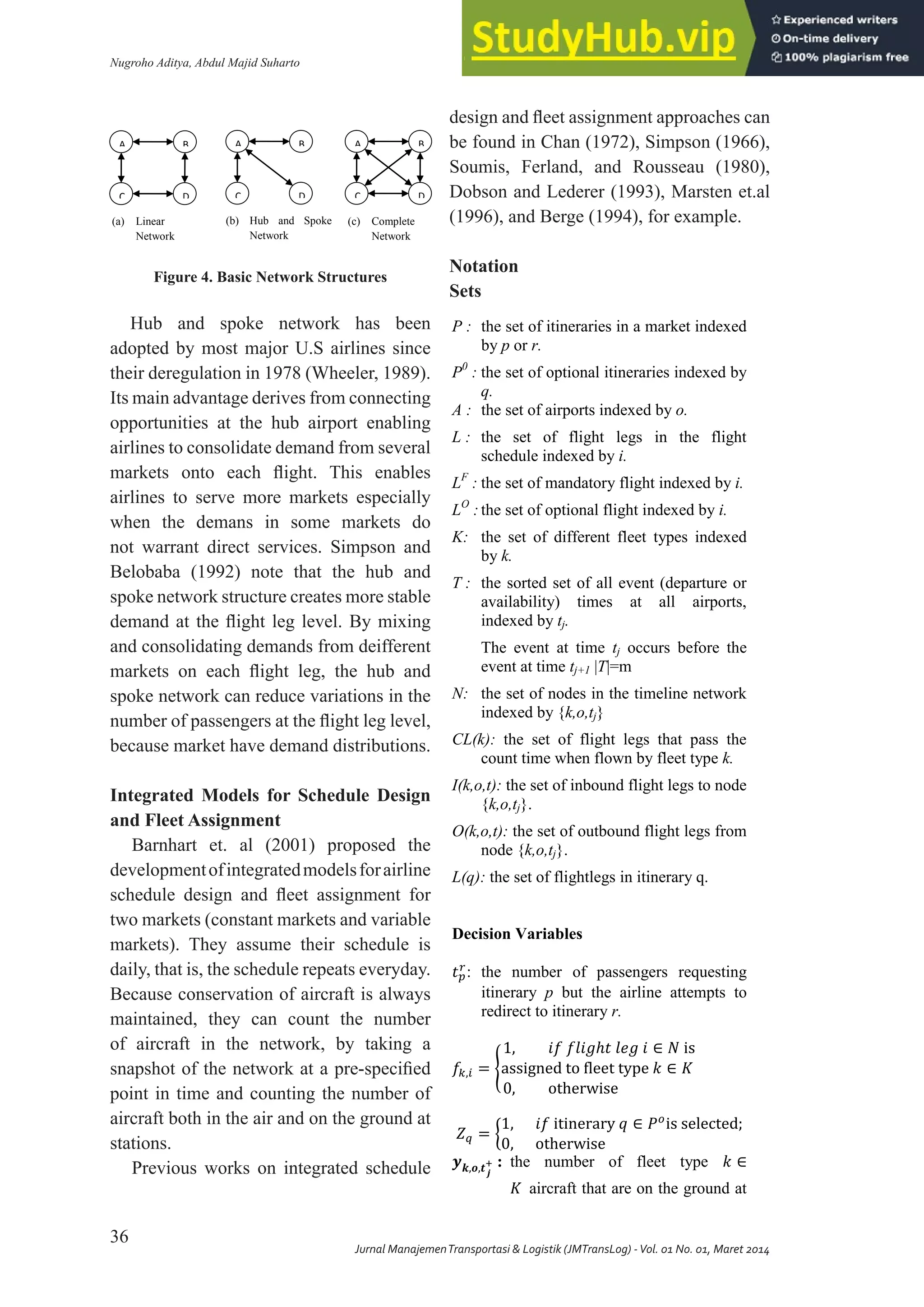
ISSN 2355-4721
to operate in all the routes. Therefore, it is
necessary to develop a new optimisation
model to solve this problem for future
work.
Notes:
This literature review was done during
the course of master degree at National
University of Singapore (NUS) as part of
project assignment for CE6001 Operation
and Management Infrastructure Systems.
He graduated from Department of Civi-
land Environmental Engineering of Na-
tional University of Singapore (NUS).
References
Abara, J. 1989. Applying Integer Linear
Programming to the FleetAssignment
Problem. Interfaces 19(4): 20-28.
Barnhart, C., Kniker, TS., & Lohatepanont,
M. 2002. Itinerary Based Airline
Fleet Assignment. Transportation
Science 36(2):199-217.
Barnhart, C., Lu, F., & Shenoi, R. 1998a.
Integrated airline schedule planning.
In: Operations Research in theAirline
Industry, G. Yu (Eds.), Kruwer
Academic Publishers: 384-403.
Barnhart, C., Belobaba, P., & Odoni, AR.
2003. Applications of Operations
Research in the Air Transport
Industry. Transportation Science 37:
368-391.
Berge, M & Hopperstad, C. 1993.
Demand Driven Dispatch: A
Method of Dynamic Aircraft
Capacity Assignments, Models and
Algorithms. Operations Research
41(1):153 - 168.
Gao, C. 2007. Airline integrated planning
and operations. [Ph.D Dissertation]
Georgia Institute of Technology.
Hane, CA., Barnhart, C., Johnson,
EL., Marsten, RE., Nemhauser,
GL., & Sigismondi, G. 1995. The
Fleet Assignment Problem: Solving
a Large Scale Integer Program.
Mathematical Programming 70:
211-232.
Lohatepanont, M & Barnhart, C. 2004.
Airline Schedule Planning: Integrated
Models and Algorithms for Schedule
Design and Fleet Assignment.
Transportation Science 38(1), 19-32.
Rushmeier, RA., Kontogiorgis, SA. 1997.
Advances in the Optimisation
of Airline Fleet Assignment.
Transportation Science 31(2): 159-
169.
Subramanian, R., Scheff, RP., Quillinan,
JD., Wiper, DS., & Marsten, R.E.
1994. Coldstart: Fleet Assignment
at Delta Air Lines. Interfaces 24(1):
104-120.

41
ISSN 2355-4721
Appendix
Figure 1 Airline Planning Process

42
ISSN 2355-4721

Airline Fleet Assignment And Schedule Planning

More Related Content

What's hot

Similar to Airline Fleet Assignment And Schedule Planning

More from Andrew Molina

Recently uploaded

Airline Fleet Assignment And Schedule Planning