Airline Fleet Assignment And Schedule Design Integrated Models And Algorithms

Airline Fleet Assignment and Schedule Design:
Integrated Models and Algorithms
by
Manoj Lohatepanont
B.Eng., Chulalongkorn University (1995)
MST, Massachusetts Institute of Technology (1999)
SM OR, Massachusetts Institute of Technology (1999)
Submitted to the Department of Civil and Environmental Engineering
in partial fulfillment of the requirements for the degree of
Doctor of Science in Transportation and Logistics Systems
at the
MASSACHUSETTS INSTITUTE OF TECHONOLOGY
February 2002
@ Massachusetts Institute of Techonology 2002
BARKER
MASSACHUSETTS iNgTITUTE
OF TECHNOLOGY
MAR 0 6 2002
LIBRARIES
Signature of Author ........................................ -.....
Department of Civil and Environmental Engineering
September 7, 2001
Certified by .......................................... . . .......................
Cynthia Barnhart
Associate Professor of Civil and Environmental Engineering
/Co-Director, Operations Research Center
C irwcty, Center for Transportation Studies
Thesis Supervisor
Accepted by ..................................................................
Oral Buyukozturk
Chairman, Departmental Committee on Graduate Studies

Airline Fleet Assignment and Schedule Design:
Integrated Models and Algorithms
by
Manoj Lohatepanont
Submitted to the Department of Civil and Environmental Engineering
on September 7, 2001, in partial fulfillment of the
requirements for the degree of
Doctor of Science in Transportation and Logistics Systems
Abstract
In scheduled passenger air transportation, airline profitability is critically influenced by the
airline's ability to construct flight schedules containing flights at desirable times in profitable
markets. In this dissertation, we study two elements of the schedule generation process, namely,
schedule design and fleet assignment. The schedule design problem involves selecting an optimal
set of flight legs to be included in the schedule, while the fleet assignment problem involves
assigning aircraft types (or fleets) to flight legs to maximize revenues and minimize operating
costs simultaneously.
With the fleet assignment problem, we investigate the issues of network effects, spill, and
recapture. On a constrained flight leg in which demand exceeds capacity, some passengers are
not accommodated, or spilled. When passengers travel on two or more constrained legs, flight
leg interdependenciesor network effects arise because spill can occur on any of these legs. In
most basic fleet assignment models, simplistic modeling of network effects and recapture leads
to sometimes severe, miscalculations of revenues. Recapture occurs when some of the spilled
passengers are re-accommodated on alternate itineraries in the system. In this dissertation, we
develop new fleet assignment models that capture network effects, spill, and recapture. Another
benefit of one of our models is its tractability and potential for further integration with other
schedule planning steps. Our study shows that the benefits of modeling these elements can be
as large as $100 million annually for a major U.S. airline. In addition, we show that modeling
flight leg interdependence is more important than demand stochasticity for hub-and-spoke fleet
assignment problems.
We develop two models for schedule design, one assuming that the market share of an airline
remains constant with schedule changes; and the other assuming that market share varies with
schedule changes. The constant market share model, while less precise in its modeling, is much
easier to solve than the variable market share model. We estimate that the potential benefits
of these models range from $100 to $350 million annually.
Thesis Supervisor: Cynthia Barnhart
Title: Associate Professor of Civil and Environmental Engineering
Co-Director, Operations Research Center
Co-Director, Center for Transportation Studies
3

Acknowledgements
My sincere gratitude goes to Professor Cynthia Barnhart for her constant understanding and
support. Her advice contributed in large measures to the success of this dissertation. She has
always been an understanding mentor and trusted friend. I have learned many valuable lessons
from her.
I sincerely thank Professors Nigel Wilson, Peter Belobaba, and John-Paul Clarke for their
invaluable advice. Their insightful comments and suggestions at the committee meetings have
contributed greatly to my dissertation.
I am grateful to the Ananda Mahidol Foundation who provides me a wonderful opportunity
to pursue my higher education here at MIT. Thanks are also due to faculty members at the
Department of Civil Engineering, Chulalongkorn University.
Many thanks go to people at United Airlines, particularly, Raj Sivakumar, Chris Spidle,
Amit Mukherjee, and Jon Goodstein, for their assistance.
I wish to thank my colleagues at MIT, notably, Tim Kniker, Andy Armacost, Amr Farahat,
Amy Mainville Cohn, Stephane Bratu, Shan Lan, and Su Shen. Their contributions to my
research are greatly appreciated. Staffs at the Center for Transportation Studies have been very
helpful and supportive. I thank Maria Marangiello, in particular, for her wonderful assistance
in all matters.
Many thanks are due to many of my friends both in Thailand and in the US, namely, Kla,
Nick, Toey, Tee+, Nog, Nam, Vijak, Jad, Berm, Isra&Sao, Chalee ,Malee, Josh, Pep, Teng, Ya,
Kung, Yot, Koi, Oy, Paan, Tao, Eak, and p'Ae. I would like to thank Boy, in particular, for
his wonderful suggestions and friendly support.
Finally, I would like to thank the most important people in my life-my family. Their
support, love, and blessing are most precious and invaluable to me. I love them all.
7

Contents
1 Introduction 19
1.1 An Overview of Airline Planning Process . . . . . . . . . . . . . . . . . . . . . . 20
1.1.1 Fleet Planning . . . . . . . . . . . . . . . . . . . . . . . . . . . . . . . . . 20
1.1.2 Schedule Planning . . . . . . . . . . . . . . . . . . . . . . . . . . . . . . . 22
1.1.3 Revenue Management . . . . . . . . . . . . . . . . . . . . . . . . . . . . . 25
1.1.4 Crew Scheduling . . . . . . . . . . . . . . . . . . . . . . . . . . . . . . . . 27
1.1.5 Airport Resource Planning . . . . . . . . . . . . . . . . . . . . . . . . . . 28
1.1.6 An Example of An Airline's Planning Process . . . . . . . . . . . . . . . . 29
1.2 Dissertation Objectives and Outline . . . . . . . . . . . . . . . . . . . . . . . . . 30
2 The Fleet Assignment Problem: An Overview 33
2.1 Introduction . . . . . . . . . . . . . . . . . . . . . . . . . . . . . . . . . . . . . . . 33
2.1.1 Outline . . . . . . . . . . . . . . . . . . . . . . . . . . . . . . . . . . . . . 33
2.2 Assumptions in Airline Fleet Assignment Models . . . . . . . . . . . . . . . . . . 34
2.2.1 Demand Issues and Assumptions in the Fleeting Process . . . . . . . . . . 34
2.2.2 Network Related Assumption . . . . . . . . . . . . . . . . . . . . . . . . . 36
2.3 Airline Fleet Assignment Literature Review . . . . . . . . . . . . . . . . . . . . . 37
2.4 Review of Airline Fleet Assignment Models . . . . . . . . . . . . . . . . . . . . . 39
2.4.1 N otation . . . . . . . . . . . . . . . . . . . . . . . . . . . . . . . . . . . . . 39
2.4.2 Input Data . . . . . . . . . . . . . . . . . . . . . . . . . . . . . . . . . . . 40
2.4.3 Fleet Assignment Model . . . . . . . . . . . . . . . . . . . . . . . . . . . . 43
2.4.4 The Fleet Assignment with Time Windows Model . . . . . . . . . . . . . 48
9

2.5 Summary . . . . . . . . . . . . . . . . . . . . . . . . . . . . . . . . . . . . . . .
3 Network Effects and Recapture in the Airline Fleet Assignment Problem 51
3.1 Introduction ........ ....................................... 51
3.1.1 Outline ........ ..................................... 52
3.2 Network Effects ........ ..................................... 52
3.3 Review of Passenger Mix and Itinerary-Based Fleet Assignment Models . . . . . 55
3.3.1 Terminology and Notation . . . . . . . . . . . . . . . . . . . . . . . . . . . 55
3.3.2 Passenger Mix Model . . . . . . . . . . . . . . . . . . . . . . . . . . . . . 58
3.3.3 Itinerary-Based Fleet Assignment Model . . . . . . . . . . . . . . . . . . . 63
3.4 Data . . .. . .
..... ..... ................. ...... ...... .... 68
3.5 Analysis of IFAM Contribution . . . . . . . . . . . . . . . . . . . . . . . . . . . . 68
3.5.1 Results and Analysis . . . . . . . . . . . . . . . . . . . . . . . . . . . . . . 69
3.6 IFAM Sensitivity . . . . . . . . . . . . . . . . . . . . . . . . . . . . . . . . . . . . 72
3.6.1 Sensitivity of Fleeting Decisions to Recapture Rates . . . . . . . . . . . . 73
3.6.2 Demand Uncertainty . . . . . . . . . . . . . . . . . . . . . . . . . . . . . . 76
3.6.3 Imperfect Control of Passenger Choices . . . . . . . . . . . . . . . . . . . 78
3.6.4 Demand Forecast Errors . . . . . . . . . . . . . . . . . . . . . . . . . . . . 79
3.7 Summary . . . . . . . . . . . . . . . . . . . . . . . . . . . . . . . . . . . . . . . . 80
4 Integrated Models for Airline Schedule Design and Fleet Assignment 83
4.1 Introduction . . . . . . . . . . . . . . . . . . . . . . . . . . . . . . . . . . . . . . . 83
4.1.1 O utline . . . . . . . . . . . . . . . . . . . . . . . . . . . . . . . . . . . . . 84
4.2 Demand and Supply Interactions . . . . . . . . . . . . . . . . . . . . . . . . . . . 84
4.3 Integrated Models for Schedule Design and Fleet Assignment: An Overview . . . 88
4.3.1 Previous Works . . . . . . . . . . . . . . . . . . . . . . . . . . . . . . . . . 88
4.3.2 Development Framework . . . . . . . . . . . . . . . . . . . . . . . . . . . . 90
4.4 Supporting Tools . . . . . . . . . . . . . . . . . . . . . . . . . . . . . . . . . . . . 93
4.4.1 Schedule Evaluation Model . . . . . . . . . . . . . . . . . . . . . . . . . . 94
4.4.2 Candidate Flight Generation Model . . . . . . . . . . . . . . . . . . . . . 94
4.5 Notation . . . . . . . . . . . . . . . . . . . . . . . . . . . . . . . . . . . . . . . . . 103
10
50

4.6 Schedule Design with Constant Market Share . . . . . . . . . . . . . . .
4.6.1 An Approximate Treatment of Demand and Supply Interactions
4.6.2 Objective Function . . . . . . . . . . . . . . . . . . . . . . . . . .
. . . . . 105
. . . . . 105
108
4.6.3 Formulation . . . . . . . . . . . . . . . . . . . . . . . . . . . . . . . . . . . 109
4.6.4 Solution Approach . . . . . . . . . . . . . . . . . . . . . . . . . . . . . . . 110
4.6.5 Computational Experiences . . . . . . . . . . . . . . . . . . . . . . . . . . 114
4.6.6 Full Size Problems . . . . . . . . . . . . . . . . . . . . . . . . . . . . . . . 117
4.7 Schedule Design with Variable Market Share . . . . . . . . . . . . . . . . . . . . 117
4.7.1 An Explicit Treatment of Demand and Supply Interactions . . . . . . . . 120
4.7.2 Objective Function . . . . . . . . . . . . . . . . . . . . . . . . . . . . . . . 122
4.7.3 Formulation . . . . . . . . . . . . . . . . . . . . . . . . . . . . . . . . . . . 123
4.7.4 Solution Approach . . . . . . . . . . . . . . . . . . . . . . .
. . . . . . . . . 125
4.7.5 Computational Experiences . . . . . . . . . . . . . . . . . . . . . . . . . . 128
4.8 Summary . . . . . . . . . . . . . . . . . . . . . . . . . . . . . . . . . . . . . . . . 128
5 Alternative Formulation for the Airline Fleet Assignment Problem
5.1 Introduction . . . . . . . . . . . . . . . . . . . . . . . . . . . . . . . . . . . . . .
5.1.1 Outline . . . . . . . . . . . . . . . . . . . . . . . . . . . . . . . . . . . .
5.2 Network Effects: A Closer Look . . . . . . . . . . . . . . . . . . . . . . . . . . .
5.2.1 Example: Consistent Passenger Flow and Flight Leg Interdependency
(Network Effects) . . . . . . . . . . . . . . . . . . . . . . . . . . . . . . .
5.2.2 Network Mapping . . . . . . . . . . . . . . . . . . . . . . . . . . . . . .
5.2.3 Binding Itineraries in the Context of the Fleet Assignment Problem . .
5.2.4 Network Partitions: Isolating Network Effects . . . . . . . . . . . . . . .
5.2.5 Summary . . . . . . . . . . . . . . . . . . . . . . . . . . . . . . . . . . .
5.3 Network Partitioning . . . . . . . . . . . . . . . . . . . . . . . . . . . . . . . . .
5.3.1 Mathematical Representation . . . . . . . . . . . . . . . . . . . . . . . .
5.3.2 Elementary, Full, and Complete Partitions . . . . . . . . . . . . . . . . .
5.4 An Alternate Formulation for the Fleet Assignment Problem . . . . . . . . . .
5.5 The Subnetwork-Based Fleet Assignment Model Formulation . . . . . . . . . .
5.5.1 Strength of SFAM Formulation . . . . . . . . . . . . . . . . . . . . . . .
131
131
. 132
132
132
134
136
. 136
139
139
139
140
140
. 143
145
11

5.6 Solution Approach . . . . . . . . . . . . . . . . . . . . . . . . . . . . . . . . . . . 145
5.6.1 Partition Construction . . . . . . . . . . . . . . . . . . . . . . . . . . . . . 145
5.6.2 Parsimonious Column Enumeration . . . . . . . . . . . . . . . . . . . . . 154
5.6.3 Solving SFAM . . . . . . . . . . . . . . . . . . . . . . . . . . . . . . . . . 155
5.7 Bounds on The Objective Function Values . . . . . . . . . . . . . . . . . . . . . . 155
5.8 Computational Experiences . . . . . . . . . . . . . . . . . . . . . . . . . . . . . . 157
5.8.1 Network Partition . . . . . . . . . . . . . . . . . . . . . . . . . . . . . . . 157
5.8.2 Problem Size . . . . . . . . . . . . . . . . . . . . . . . . . . . . . . . . . . 158
5.8.3 Runtime . . . . . . . . . . . . . . . . . . . . . . . . . . . . . . . . . . . . . 158
5.8.4 Contribution . . . . . . . . . . . . . . . . . . . . . . . . . . . . . . . . . . 161
5.8.5 Actual Cross-Network Error . . . . . . . . . . . . . . . . . . . . . . . . . . 162
5.8.6 Strength of Formulation . . . . . . . . . . . . . . . . . . . . . . . . . . . . 164
5.9 Summary . . . . . . . . . . . . . . . . . . . . . . . . . . . . . . . . . . . . . . . . 164
6 Subnetwork-Based Fleet Assignment Model Extensions 167
6.1 Introduction . . . . . . . . . . . . . . . . . . . . . . . . . . . . . . . . . . . . . . . 167
6.1.1 Outline . . . . . . . . . . . . . . . . . . . . . . . . . . . . . . . . . . . . . 167
6.2 SFAM with Recapture . . . . . . . . . . . . . . . . . . . . . . . . . . . . . . . . . 168
6.2.1 Modeling Recapture in SFAM . . . . . . . . . . . . . . . . . . . . . . . . . 168
6.2.2 Building Network Partitions for SFAM with Recapture . . . . . . . . . . . 170
6.2.3 SFAM with Recapture: Formulation and Solution Algorithm . . . . . . . 172
6.3 An Alternate Modeling Approach for Recapture . . . . . . . . . . . . . . . . . . . 173
6.4 SFAM in the Context of Schedule Design . . . . . . . . . . . . . . . . . . . . . . 176
6.4.1 The Schedule Design Problem with Constant Market Share . . . . . . . . 176
7 Conclusions 179
7.1 Summary of Contributions. . . . . . . . . . . . . . . . . . . . . . . . . . . . . . . 179
7.1.1 Fleet Assignment . . . . . . . . . . . . . . . . . . . . . . . . . . . . . . . . 179
7.1.2 Schedule Design . . . . . . . . . . . . . . . . . . . . . . . . . . . . . . . . 181
7.2 Directions for Future Research . . . . . . . . . . . . . . . . . . . . . . . . . . . . 182
7.2.1 Integrated Schedule Design and Fleet Assignment . . . . . . . . . . . . . 182
12

7.2.2 Multiple Fare Class Models . . . . . . . . . . . . . . . . . . . . . . . . . . 183
7.2.3 Subnetwork Based Fleet Assignment . . . . . . . . . . . . . . . . . . . . . 183
7.3 Final Thoughts . . . . . . . . . . . . . . . . . . . . . . . . . . . . . . . . . . . . . 185
A Glossary 193
13

List of Figures
1-1
1-2
An Overview of Airline Planning Process . . . . . . . . . . . . . . . . . . . . . .
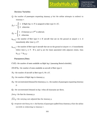
The Domestic Aircraft Scheduling Process at a Major U.S. Carrier [Adapted
from Goodstein (1997)] . . . . . . . . . . . . . . . . . . . . . . . . . . . . . . . .
2-1 Unconstrained Leg Level Demand Distribution . . . . . . . . . . . . . . . . . . .
2-2 Constrained (Observed) Leg Level Demand Distribution . . . . . . . . . . . . . .
3-1 The direct solution approach for the combined fleet assignment and passenger
mix model . . . . . . . . . . . . . . . . . . . . . . . . . . . . . . . . . . . . . . . .
3-2 Methodology . . . . . . . . . . . . . . . . . . . . . . . . . . . . . . .
3-3 Evaluation of Impacts of Recapture and Network Effects . . . . . . .
3-4 Methodology for Testing Model Senstitivity to Recapture Rate . . .
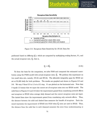
3-5 Recapture Rate Sensitivity for 1N-3A Data Set . . . . . . . . . . . .
3-6 Recapture Rate Sensitivity for 2N-3A Data Set . . . . . . . . . . . .
3-7 Methodology for Simulation 1 (Measuring the Performance of FAM
under simulated environment) . . . . . . . . . . . . . . . . . . . . . .
3-8 Model Sensitivity to Forecast Errors for Problem 1N-3A . . . . . . .
3-9 Model Sensitivity to Forecast Errors for Problem 2N-3A . . . . . . .
and IFAM
Basic Network Structures for n = 4 Cities and n(n - 1) Markets . . . .
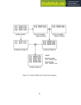
Master Flight List Construction Diagram . . . . . . . . . . . . . . . . .
An Outline of the Proposed Candidate Flight Generation Process . . . .
Market Categorization Matrix . . . . . . . . . . . . . . . . . . . . . . . .
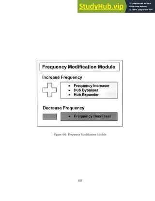
Proposed Modification Mapping . . . . . . . . . . . . . . . . . . . . . . .
. . . . . 87
. . . . . 92
. . . . . 95
. . . . . 98
. . . . . 100
15
21
30
36
37
67
69
70
73
74
75
76
80
81
4-1
4-2
4-3
4-4
4-5

4-6 Frequency Modification Module . . . . . . . . . . . . . . . . . . . . . . . . . . . . 102
4-7 Indirect Effect of Recapture Rate and Capacity Constraint on Effective Market
Share ......... ........................... ... .......... 106
4-8 The Approximate Solution Approach . . . . . . . . . . . . . . . . . . . . . . . . . 112
4-9 The solution algorithm for ISD-FAM . . . . . . . . . . . . . . . . . . . . . . . . . 113
4-10 Testing Methodology . . . . . . . . . . . . . . . . . . . . . . . . . . . . . . . . . . 116
4-11 Our Approach for Capturing Demand and Supply Interaction . . . . . . . . . . . 120
4-12 The Exact Solution Approach . . . . . . . . . . . . . . . . . . . . . . . . . . . . . 126
5-1 An Illustrative Network for Understanding Network Effects . . . . . . . . . . . . 133
5-2 An Example of Network Mapping . . . . . . . . . . . . . . . . . . . . . . . . . . . 135
5-3 Network Partition . . . . . . . . . . . . . . . . . . . . . . . . . . . . . . . . . . . 138
5-4 Graphical Representation of the Sufficiently Complete Partition in Two Full-Size
Data Sets . . . . . . . . . . . . . .. . . . . . . . .. . . . . . . . . . . . . . . . . . 147
5-5 Graphical Representation of Our Approach . . . . . . . . . . . . . . . . . . . . . 148
5-6 Subdividing a Subnetwork by Breaking the Potentially Binding Connection . . . 149
5-7 Breaking A Potentially Binding Itinerary . . . . . . . . . . . . . . . . . . . . . . 151
5-8 Three Levels of Possible Subnetwork Division . . . . . . . . . . . . . . . . . . . . 152
5-9 Bounds on Objective Function Value of SFAM . . . . . . . . . . . . . . . . . . . 156
6-1 An Example of Network Partition that Does Not Allow Effective Modeling of
Recapture ........ .......................... ............ .169
6-2 A Conceptual Diagram for Modeling Recapture Externally in the Fleeting Process174
16

List of Tables
2.1 Flight Connection Example . . . . . . . . . . . . . . . . . . . . . . . . . . . . . . 48
3.1 Demand data . . . . . . . . . . . . . . . . . . . . . . . . . . . . . . . . . . . . . . 52
3.2 Seating Capacity . . . . . . . . . . . . . . . . . . . . . . . . . . . . . . . . . . . . 53
3.3 Operating costs . . . . . . . . . . . . . . . . . . . . . . . . . . . . . . . . . . . . . 54
3.4 Possible fleeting configurations . . . . . . . . . . . . . . . . . . . . . . . . . . . . 54
3.5 The minimum spill costs and resulting contributions for each fleeting combination 54
3.6 The contribution using a greedy algorithm . . . . . . . . . . . . . . . . . . . . . . 54
3.7 PMM Model Example: Flight Schedule . . . . . . . . . . . . . . . . . . . . . . . 59
3.8 PMM Model Example: Itinerary Level Demand . . . . . . . . . . . . . . . . . . . 59
3.9 The characteristics of the data sets . . . . . . . . . . . . . . . . . . . . . . . . . . 68
3.10 The improvement in the fleeting contribution for data set 1N-9 in dollars per day
compared to basic FAM. . . . . . . . . . . . . . . . . . . . . . . . . . . . . . . . . 70
3.11 The improvement in the fleeting contribution for data set 2N-9 in dollars per day
compared to basic FAM. . . . . . . . . . . . . . . . . . . . . . . . . . . . . . . . . 70
3.12 The changes in average fare paid and average spill fare compared to basic FAM. 71
3.13 Comparison of the Performance of FAM and IFAM in Simulation 1 ($/day).... 77
3.14 Comparison of the Performance of FAM and IFAM in Simulation 2 ($/day).. . . 78
4.1 Data Characteristics . . . . . . . . . . . . . . . . . . . . . . . . . . . . . . . . . . 115
4.2 Contribution Comparision . . . . . . . . . . . . . . . . . . . . . . . . . . . . . . . 118
4.3 Problem Sizes (RMP's) and Solution Times . . . . . . . . . . . . . . . . . . . . . 118
4.4 Resulting Schedule Characteristics . . . . . . . . . . . . . . . . . . . . . . . . . . 118
17

4.5 Data Characteristics . . . . . . . . . . . . . . . . . . . . . . . . . . . . . . . . . . 118
4.6 Contribution Comparison . . . . . . . . . . . . . . . . . . . . . . . . . . . . . . . 119
4.9 Contribution Comparison . . . . . . . . . . . . . . . . . . . . . . . . . . . . . . . 127
5.1 Examples of Consistent Passenger Flows . . . . . . . . . . . . . . . . . . . . . . . 134
5.2 Leg-Level Demand . . . . . . . . . . . . . . . . . . . . . . . . . . . . . . . . . . . 136
5.3 Number of Potentially Binding Itineraries in Full Size Data Sets . . . . . . . . . 137
5.4 Itinerary D ata . . . . . . . . . . . . . . . . . . . . . . . . . . . . . . . . . . . . . 142
5.5 Fleet Type Data . . . . . . . . . . . . . . . . . . . . . . . . . . . . . . . . . . . . 142
5.6 Example of Composite Variables . . . . . . . . . . . . . . . . . . . . . . . . . . . 146
5.7 Sufficiently Complete Partition . . . . . . . . . . . . . . . . . . . . . . . . . . . . 146
5.8 Example of Composite Variables . . . . . . . . . . . . . . . . . . . . . . . . . . . 154
5.9 The characteristics of the data sets . . . . . . . . . . . . . . . . . . . . . . . . . . 157
5.10 Network Partitions for Data Set 1N-9 . . . . . . . . . . . . . . . . . . . . . . . . 157
5.11 Network Partitions for Data Set 2N-9 . . . . . . . . . . . . . . . . . . . . . . . . 158
5.12 Problem Sizes for Data Set 1N-9 . . . . . . . . . . . . . . . . . . . . . . . . . . . 159
5.13 Problem Sizes for Data Set 2N-9 . . . . . . . . . . . . . . . . . . . . . . . . . . . 159
5.14 Runtimes (sec) for Data Set 1N-9 . . . . . . . . . . . . . . . . . . . . . . . . . . . 160
5.15 Runtimes (sec) for Data Set 2N-9 . . . . . . . . . . . . . . . . . . . . . . . . . . . 160
5.16 Contributions ($/day) for Data Set 1N-9 . . . . . . . . . . . . . . . . . . . . . . . 161
5.17 Contributions ($/day) for Data Set 2N-9 . . . . . . . . . . . . . . . . . . . . . . . 163
5.18 Actual Cross-Network Errors ($/day) for Data Set 1N-9 . . . . . . . . . . . . . . 163
5.19 Difference between the Root Node LP Relaxation and Best IP Solutions ($/day) 164
18

Chapter 1
Introduction
markets (defined by origin-destination pairs). Airlines engage in a complex decision making
process generally referred to as airline schedule planning, which is comprised of many tasks
(detailed in Section 1.1), in order to produce operational schedules. Generating an optimal
schedule for any given period is of utmost interest and importance to the airlines. In the past,
these tasks are divided and optimized in a sequential manner because the integrated model to
optimize the entire process is enormous and unsolvable. Today, advanced technologies and
better understanding of the problems have allowed operations researchers to begin integrating
and globally optimizing these sequential tasks.
In this dissertation, we are interested in particular in the airline schedule design and fleet
assignment problems. The schedule design problem involves selecting an optimal set of flight
legs to be included in the schedule based on forecasted demand, while the fleet assignment
problem involves optimally assigning aircraft types to flight legs to maximize revenue and
minimize operating cost. We review and validate existing fleet assignment models and present
a new approach. Based on the knowledge of the fleet assignment problem, we propose new
approaches to integrate the airline schedule design and fleet assignment problems.
19

1.1 An Overview of Airline Planning Process
In order to facilitate the comprehension of this complex decision making process, we refer to
Figure 1-1, which simplifies the airlineplanning process into several sequential steps. On the
left axis of Figure 1-1, the vertical bar describes the time horizon of this sequential process
from several years out to a few days before flight departures. The right axis categorizes the
nature of the decisions involved in this planning process, ranging from strategic at the top down
to tactical/operational decisions at the bottom. Note, however, that different approaches are
taken at different airlines; thus, the steps depicted in Figure 1-1 should be interpreted only as
a representative approach.
1.1.1 Fleet Planning
The first step in creating an operational airline schedule is fleet planning, in which the airline
decides how many and what types of aircraft it should acquire, either through buying or leas-
ing. Fleet planning is one of the most important strategic decisions and involves huge capital
investment. Major fleet planning is done infrequently and each decision has long lasting ef-
fects and implications that will greatly affect, or often times restrict, the downstream planning
process. Minor revision of the fleet planning is done more frequently and often affects only a
small number of aircraft. There are two major approaches to fleet planning (Belobaba, 1999):
1. "Top-Down" Approach, and
2. "Bottom-Up" Approach.
The "top-down" approach involves high level, system wide financial analysis of the impacts
of options. It typically utilizes system level estimates of demand, revenue, and aggregate
cost information. This approach is most common in practice because it does not involve
sophisticated models or detailed analysis, requiring a full range of assumptions and unreliable
forecasts, for uncertain 5 - 15 year scenarios.
The "bottom-up" approach, however, goes through a series of detailed simulations of airline
operations, ranging from route structure to operations. This approach depends heavily on the
quality of the data, especially the detailed forecasts of future scenarios.
20

.o Schedule Design
o Fleet Assignment
0 Aircraft Rotations
F* i 0
Revenue Crew Scheduling
Management
- Pricing
- Seat Inventory Airport Resource
ControlPlanning
Figure 1-1: An Overview of Airline Planning Process
21

Vaysse (1998) presents an example of models in the "bottom up" family. Her approach can
be decomposed into two dimensions; namely, single-period demand allocation and multi-period
fleet optimization. The former focuses on allocations of passengers to schedules, maximizing
potential profitability. The latter focuses on optimal assignments of aircraft types to schedules
from different periods, minimizing operating cost and maintaining consistency of fleet family.
Once an airline selects particular fleets, it often commits to them for a very long period
of time. Thus, most of the time, the rest of the planning process will take as given the fleet
family. There has not been efforts to integrate fully the fleet planning decision into the rest
of the planning process because the time horizon involved in fleet planning differs greatly from
the rest of the planning process. Thus, in this paper, we will also assume that the fleet
composition of the airline is given. Note, however, that some of the tools developed for the
rest of the planning process, in particular, those for the schedule design and fleet assignment
steps, can be adapted and used for fleet planning purposes, as we will explain later.
1.1.2 Schedule Planning
The schedule planning step typically begins 12 months before the schedule goes into operation
and lasts approximately 9 months. Airlines spend a great amount of time and resource in
this step in order to come up with a competitive and profitable schedule. In the beginning,
the schedule planning step begins with route development, in which the airline decides which
markets, defined by origins and destinations, it wants to serve, based primarily on system-wide
demand information. Major route developments are done infrequently, typically at the launch
of the airline operation and afterwards in major route revisions, such as the introduction of
a new hub . Most of the time, the schedule planning step starts from an existing schedule,
with a well developed route structure. Changes are then introduced to the existing schedule to
reflect changing demands and environment; this is referred to as schedule development. There
are three major components in the schedule development step:
1. Schedule Design,
2. Fleet Assignment, and
3. Aircraft Rotations.
22

As pointed out earlier, these sequential steps should not be interpreted as a standard, rather
they facilitate our understanding of the process. Different airlines have different tools, culture,
and management styles, and therefore, the actual implementations may differ in the details.
Schedule Design
The schedule design step is arguably the most complicated step of all and traditionally has been
decomposed into two sequential steps:
1. frequency planning, and
2. timetable development.
In frequency planning, planners determine the appropriate service frequency in a market.
In timetable development, planners place the proposed services throughout the day subject to
approximate network considerations and other constraints.
Frequency Planning. The objective of frequency planning is to match daily or weekly fre-
quency to the anticipated demand in every market ensuring that the level of demand anticipated
and the frequency are balanced and reasonable. This depends on many market-dependent
factors, such as length of haul and market type, for example. If the market is a long-haul inter-
national market, the airline might be able to offer only a limited number of flights daily, while
in a popular short haul domestic market, hourly flight offerings are common. If the market is
composed heavily of business travelers, then schedule convenience measured in terms of flight
availability is important, and thus, frequent flight offerings are necessary to build presence in
the market. On the other hand, if the market is composed primarily of leisure travelers, flight
availability is of lesser importance and high levels of frequency are not necessary.
Teodorovic and Krcmar-Nozic (1989) present a methodology that determines optimal flight
frequencies on a network maximizing total profit and market share and minimizing the total
schedule delay of all passengers on the network. They incorporate approximate vehicle consid-
erations by setting a maximum number of services in each market and a maximum number of
seat-hours (a measure of an airline's production level) for the entire system.
23

Timetable Development. After the airline decides how many flights it wants to offer in each
market, the next step is to decide at what times should these flight be offered. This depends
on market characteristics as well as schedule constraints. For example, in business markets,
hourly flight offerings are desired because it gives business travelers both schedule availability
and reliability. The departure times of these flights, however, have to be synchronized such
that the schedule is (or potentially is) flyable by the available number of aircraft.
Berge (1994) presents a sub-timetable optimization approach, in which sub-timetable, a
small part of the network, is optimized and augmented to the master (existing) timetable.
The sub-timetable optimization model takes as input, among other things, a list of candidate
flight legs specified by origin, destination, departure and arrival times. The model optimized
the schedule by selecting flight legs that maximize market coverage, the probability that a
random passenger finds at least one path, i.e., a sequence of flight legs from origin to ultimate
destination, in his/her decision window. Full scale timetable optimization is still not feasible
currently because of its size and complexity (Belobaba, 1999).
Fleet Assignment
The purpose of fleet assignment is to assign the available aircraft to every flight leg such that
the seating capacity on the aircraft closely matches the demand for every flight. If too small an
aircraft is assigned to a particular flight, many potential passengers are turned away, or spilled,
resulting in potential lost revenue. On the other hand, if too big an aircraft is assigned to a
particular flight, many empty seats, which can potentially be utilized more profitably elsewhere,
are flown. The assignment of aircraft to flight legs has to respect conservation of aircraft flow,
that is, an aircraft entering a station has to leave that station at some later point in time. The
airlines cannot assign more aircraft than are available. If the schedule cannot be fleeted with
the available number of aircraft, minor changes must be made to the schedule.
Dantzig (1954), Daskin and Panayotopoulos (1989), Abara (1989), Hane et al. (1995),
Rexing et al. (2000), Barnhart, Kniker, and Lohatepanont (2001), and Jacobs, Smith and
Johnson (2000) study the fleet assignment problem from many aspects. The fleet assignment
with time windows model by Rexing et al. (2000), in particular, allow minor re-timing of flight
legs, thus potentially allowing otherwise infeasible schedules to be fleeted. The itinerary-based
24

fleet assignment model by Barnhart, Kniker, and Lohatepanont (2001) improves upon the basic
fleet assignment model by Hane et al.(1995), by considering network effects and recapture.
Network effect refers to the problem of inconsistent passenger flow that might occur because of
flight leg independence assumptions in the basic fleet assignment model. Recapture happens
when some of the otherwise spilled passengers are recaptured by the airline on other flight legs
in the system.
Aircraft Rotations
The objective of the aircraft rotation step is to find a maintenance feasible rotation (or rout-
ing) of aircraft, given a fleeted schedule (from the previous step) and the available number of
aircraft of each type. A rotation is a sequence of connected flight legs that are assigned to a
specific aircraft, beginning and ending at the same location, over a specific period of time. A
maintenance feasible rotation is a routing of an aircraft that respects the maintenance rules of
the airlines and regulatory agencies.
Note that in many fleet assignment models (for example, Hane et al 1995, and Clarke et
al 1996), maintenance requirements are modeled only approximately by ensuring a sufficient
number of maintenance opportunities for each fleet type. A maintenance opportunity exists
when an aircraft overnights at one of its maintenance locations. While this ensures that, on
average, enough aircraft of each type are in maintenance nightly, it does not guarantee that
individual aircraft are treated equally: one aircraft might have one maintenance opportunity
per day while another might not have any in a week. The aircraft maintenance routing problem
addresses this issue in detail.
Simpson (1969) reviews several models for the aircraft routing problem. Recent works in
this area include Gopalan and Talluri (1993), Clarke et al. (1996), and Barnhart et al. (1997).
In Barnhart et al. (1997), maintenance routing is integrated with fleet assignment and applied
to an application involving a long-haul flight schedule.
1.1.3 Revenue Management
Given a fleeted schedule, the objective of revenue management is to maximize revenue. An ideal
revenue management system consists of two distinct but closely related components (Belobaba,
25

1987):
1. differential pricing, and
2. seat inventory control.
Pricing
After deregulation in 1978, the airline industry has evolved significantly from an industry with
very stable pricing to one with a volatile and complicated pricing structure. Most airlines now
practice price differentiation,that is, offering different "fare products" with different restrictions
at different prices (Belobaba, 1999). This concept fully takes advantage of the economic concept
of passenger "willingness to pay1
". The differential price offering aims to stimulate demand
with low fare offerings and to capture the willingness to pay of high fare passengers. Fare
restrictions attempt to prevent demand dilution from diversion-the pattern of existing high
fare passengers opt to take advantage of low fare offering.
There are a number of papers in this area, including, for example, Oum, Zhang, and Zhang
(1993), Weatherford (1994), Gallego (1996), and Gallego and Van Ryzin (1997).
Seat Inventory Control
The objective of seat inventory control is to determine the number of seats on a flight to be
made available to a particular fare product. The idea is to limit low-fare seats and protect
higher-fare seats for later-booking passengers. Airlines utilize a set of tools to achieve this
objective (Belobaba, 1992):
1. overbooking: acceptance of bookings in excess of capacity to minimize the potential empty
seats on board,
2. fare class mix: limiting the availability of seats sold at various price levels on a flight leg;
and
1 In short, the same product can be sold for different prices to different consumers based on the values that
the consumers associate with the product. If the product is of higher value to a consumer, the producer would
charge a higher price knowing that he/she would pay for it. On the other hand, if the product is of lesser value
to another customer, the producer would alternatively charge a lower price to that customer. In an ideal world,
if the producer could charge each customer the highest price he/she would be willing to pay, the producer's profit
would be maximized.
26

3. itinerary control: discrimination among passengers traveling on different multiple leg
itineraries.
Overbooking and fare class mix have been the focus of early revenue management efforts
(see Belobaba, 1989, 1992, Curry, 1990, Brumelle et al., 1990, and Wollmer, 1992, for example).
Recent development is progressing towards origin-destination or network level inventory control,
that is, a move towards incorporating itinerary control (see, for example, Simpson, 1989, Smith
et al., 1992, Williamson, 1992, and Bratu, 1999).
One of the most crucial inputs for any seat inventory control practice is the forecasted
demand. The level of detail differs for each model, ranging from leg-based fare classes to
origin-destination-based fare classes (see, for example, Heureux, 1986, Lee, 1990, Gallego, 1996,
and Kambour, Sivaramakrishnan, and Boyd, 2000).
Clearly there are many potential benefits to be gained from integrating pricing and seat
inventory control into one seamless revenue management system (Marcotte and Savard, 2000,
and Lieberman, 2000). Surprisingly, these tasks are still performed separately at most airlines,
often by different departments. This arises partly because of the dominant practice in airline
pricing of "matching" fares offered by competitors (Belobaba, 1987).
1.1.4 Crew Scheduling
In crew scheduling, the objective is to find the minimum cost assignment of flight crews (pilots
and/or flight attendants) to flight legs subject to several restrictions, some of which are: pilots
are qualified to fly only certain aircraft types; work schedules must satisfy maximum time-away-
from- base (the period that flight crews are away from their domicile stations) restrictions;
crews are not allowed to stay on duty longer than a maximum flying time requirement; and
work schedules must satisfy minimum rest time. Crew scheduling is typically broken into two
steps (Barnhart and Talluri, 1996):
1. the crew pairingproblem, and
2. the crew assignment problem.
The objective of the crew pairing problem is to find a set of work schedules that cover
each flight the appropriate number of times and minimize total crew costs. Crew pairing
27

problems are usually formulated as Set Partitioningproblems where each row corresponds to
a scheduled flight and each column corresponds to a legal crew pairing (1997). A pairing is
composed of duties, separated by rest periods. A duty is a sequence of flight legs to be flown
consecutively in one day that satisfies all work rules. In some instances, deadheading (flight
crews being repositioned by flying as passengers) is allowed. Deadheading can be advantageous,
especially in long-haul crew pairing problems as shown by Barnhart et al. (1995). Vance et
al. (1994) present a formulation for crew pairing optimization with decision variables based on
duty periods rather than pairings. Subramanian and Marsten (1994) present an integrated
model for the fleet assignment and crew pairing problems.
In crew assignment, these pairings are combined with rest periods, vacations, training time,
etc., to create extended work schedules that can be performed by an individual. The objective
of the crew assignment problem is to find a minimum cost assignment of employees to these
work schedules. There are two traditional approaches for crew assignment:
1. rostering,and
2. bidline generation.
With rostering, a common practice in Europe, schedules are constructed for specific individ-
uals. A subset of schedules is selected such that each individual is assigned to a schedule, and all
pairings in the crew pairing problem solution are contained in the appropriate number of sched-
ules. With bidline generation, a common practice in North America, the cost-minimizing subset
of schedules is selected without referring to specific individuals. Employees then reveal their
relative preferences for these schedules through a bidding process. The airline assigns schedules
to employees based on individual priority rankings, which are often related to seniority.
1.1.5 Airport Resource Planning
Primary tasks that are done in the airport resource planning step are gate allocation, slot al-
location (if applicable), and ground personnel scheduling. Gate allocation involves assigning
available gates at stations to arriving and departing aircraft such that all flight legs are covered,
aircraft servicing can be accomplished, and passenger connections can be made within reason-
28

able amounts of time. See, for example, Mangoubi and Mathaisel (1984), Vanlaningham and
West (1988), and Richardson (1991).
Slot allocation is closely related to gate allocation but only applies to slot controlled airports.
In the U.S., these are Washington National, New York J.F.K., New York LaGuardia, and
Chicago O'Hare airports. At these airports, the number of takeoffs and landings (slots) is
controlled by regulatory agencies in order to alleviate flight delay problems resulting from
congestion. Slots are allocated, by an allocation committee, in advance, to carriers serving
these airports. Airlines have to schedule according to the slots allocated, which must be
synchronized with gate allocation and incorporated into the schedule building process in order
to avoid potential infeasibilities or violations.
Ground personnel scheduling involves scheduling staff to several airport ground positions,
including check-in agents, gate agents, aircraft servicing staff, luggage handling staff, and field
staff. See for example, Buch (1994), and White (1997).
1.1.6 An Example of An Airline's Planning Process
Figure 1-2 depicts the domestic aircraft scheduling process at a major U.S. carrier (Goodstein,
1997). The fleet planning and route development processes begin as much as 5 years before
the departure date. The period from one year to 52 days before the departure date is divided
into three phases:
1. Schedule Planning (1 year to 108 days before the departure date),
2. Intermediate Scheduling (108 to 80 days before the departure date), and
3. CurrentScheduling (80 to 52 days before the departure date).
In Schedule Planning, planners prepare a schedule for the next period by modifying existing
schedules. This step requires a relatively long amount of time to perform because of the com-
plexity involved. At this step, operational constraints are incorporated only approximately.
Once a schedule is developed, the Intermediate Scheduling group begins to investigate the op-
erational feasibility of the proposed schedule in terms of fleet assignment, maintenance routing,
crew scheduling, etc. Revenue management begins when the schedule goes into the Current
29

S
5
years
1
year
Interm
Sche
chedul
lannin
Current
Scheduling
ediate
duling
e
g
108
days
80
days
52
days
Profit Focus
Operational Feasibility Focus
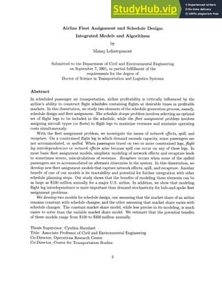
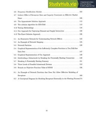
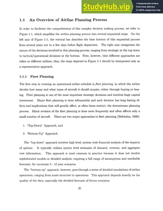
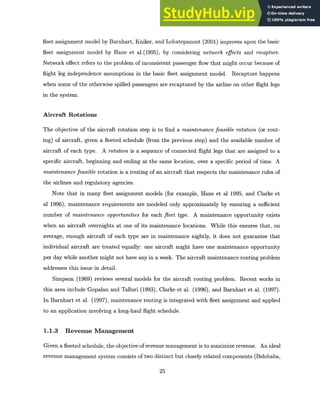
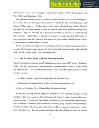
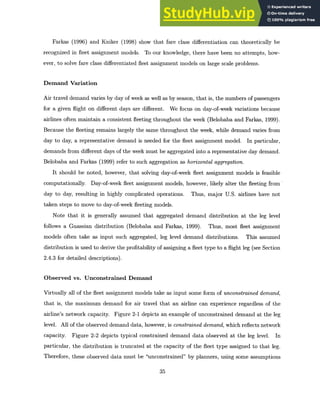
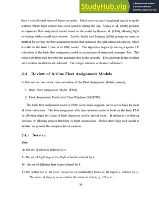
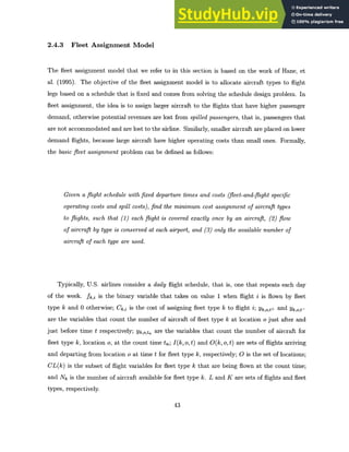
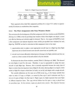
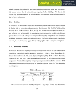
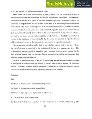
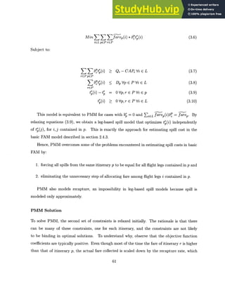
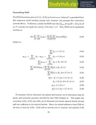
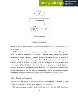
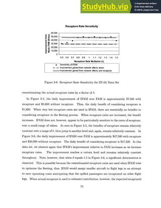
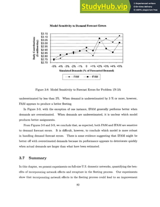
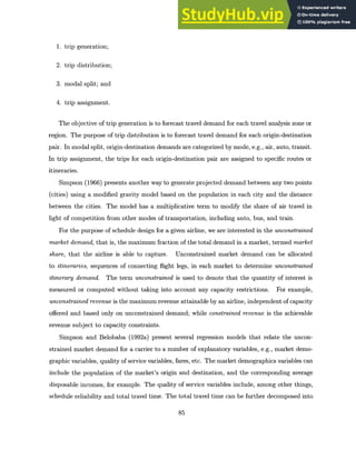
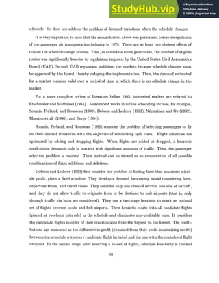
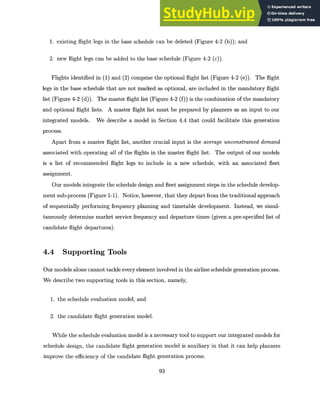
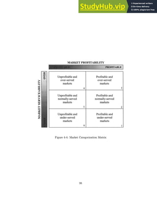
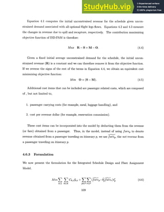
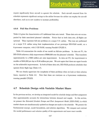
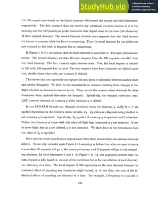
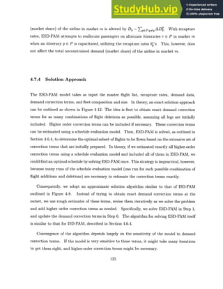
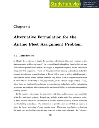
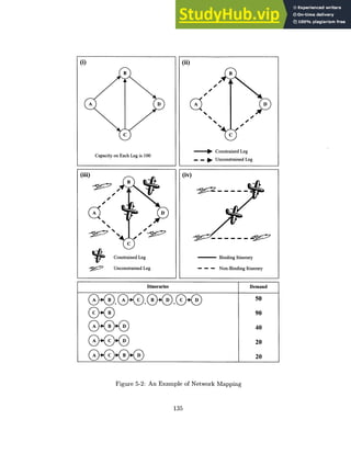
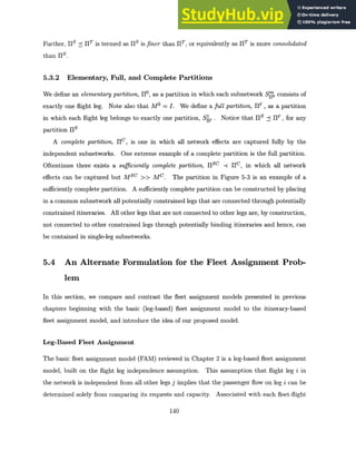
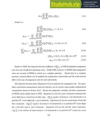
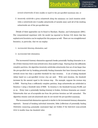
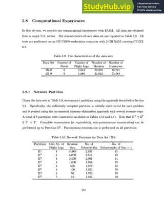
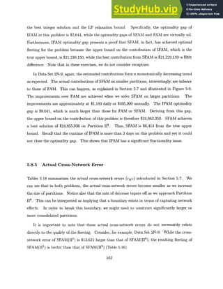
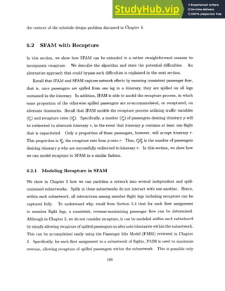
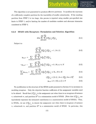
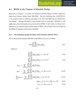
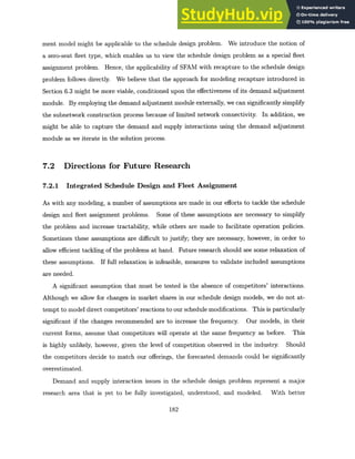
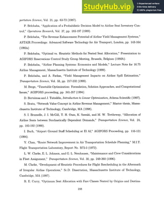
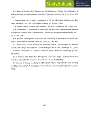
Figure 1-2: The Domestic Aircraft Scheduling Process at a Major U.S. Carrier [Adapted from
Goodstein (1997)]
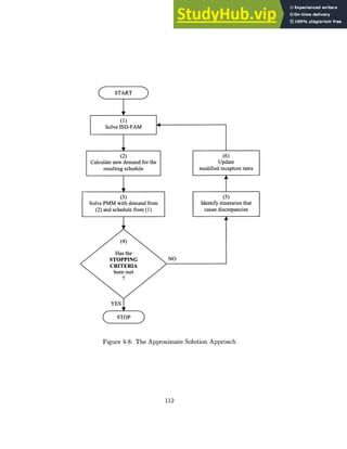
Scheduling phase. Minor changes can be made to the planned schedule as additional data be-
come available. Demand data is of particular interest because re-fleeting models (Goodstein,
1997) are available to modify the fleeting decisions slightly in order better to match capacity
with demand, as the departure date approaches. Notice also that the focus or objectives of
planners shift from profitability maximization to operational feasibility as we move from the
early stages of planning to the departure date.
1.2 Dissertation Objectives and Outline
Earlier in this chapter, we present a detail overview of the airline planning process. In this
dissertation, our primary focus is on schedule design and fleet assignment. In Chapter 2, we
present an extended review of the fleeting process. In particular,
1. modeling assumptions of most fleet assignment models are explained in detail;
2. we present relevant literature on airline fleet assignment; and
30
r-

3. we review basic fleet assignment models.
In Chapter 3, we review an enhanced fleet assignment model, the itinerary-based fleet
assignment model (Barnhart, Kniker, and Lohatepanont, 2001), which we use to study the
influence of network effects and recapture in the fleeting process. Network effects refer to the
phenomenon in which flight legs in the network interact when passengers travel on more than
one leg. Recapture occurs when some of the otherwise spilled passengers are re-accommodated
on alternate itineraries in the system. We present a set of experiments designed to validate
several assumptions used in this enhanced model.
Integration of the fleeting and schedule design processes is of particular interest to us and will
be accomplished by extending the itinerary-based fleet assignment model (Barnhart, Kniker,
and Lohatepanont, 2001). Two models will be developed, in Chapter 4, based on two different
models of airline market share:
1. Constant Market Share, and
2. Variable Market Share.
In the constant market share case, we assume that the market share of the airline remains
constant with schedule changes; whereas in the variable market share case, the market share
of the airline changes with schedule changes. While the constant market share assumption
might not be accurate under all scenarios, we will demonstrate its applicability. Its advantage
is its superior tractability relative to variable market share models. We will investigate the
performance of variable market share models under other scenarios, and report computational
results.
We revisit the issue of network effects in the fleeting process in Chapter 5. We are inter-
ested in understanding how network effects arise and how exactly flight legs interact with each
other. Based on this knowledge, we present a new approach for solving the fleet assignment
problem. It attempts to model passenger flow more accurately without explicitly considering
actual passenger flow variables. The model formulation and solution algorithms are presented.
The primary advantage of this approach is its potential to integrate with other airline planning
problems, such as schedule design or aircraft maintenance routing. In Chapter 6, we discuss
31

some possible extensions of our new fleeting model presented in Chapter 5. The extensions
include recapture and application to the schedule design problem. Finally, in Chapter 7, we
present a summary of contributions and directions for future research.
32

Chapter 2
The Fleet Assignment Problem: An
Overview
2.1 Introduction
In general, the fleet assignment problem involves assigning available aircraft to flight legs such
that revenue is maximized and simultaneously operating cost is minimized. Although the
application of operations research techniques to the fleet assignment problem can be traced
as far back as 1954 by Dantzig and Ferguson (1954), there are many aspects of the problem
that are yet to be investigated thoroughly. In this chapter we describe some of the underlying
assumptions used in most fleet assignment models and provide a review of recent literature.
Two basic fleet assignment models are reviewed to provide a basis for our discussions in the
remainder of this dissertation.
2.1.1 Outline
In Section 2.2, we detail some of the assumptions used in most fleet assignment models. Next,
in Section 2.3, we review the airline fleet assignment literature. We present one of the most
basic formulations for the fleet assignment problem and an extension in Section 2.4. Finally,
we provide concluding remarks in Section 2.5.
33

2.2 Assumptions in Airline Fleet Assignment Models
Recall from Figure 1-2 that airlines start the fleeting process long before the schedule become
effective. One could imagine that there are many uncertainties that could affect the selected
fleeting. Major airlines, however, cannot afford to wait until the very last minute until every-
thing is more certain to start planning their schedule because of the scale and complexity of
their operations. Therefore, assumptions have to be made to allow getting the planning process
started. Additional assumptions might be needed as well from a modeling standpoint. In this
section, we discuss those assumptions underlying the airline fleet assignment process.
2.2.1 Demand Issues and Assumptions in the Fleeting Process
Every fleet assignment model requires as input an estimate of demand at flight leg or itinerary
level. In this section, we discuss how such demand forecasts can be developed, focusing on the
underlying assumptions. There are a number of factors that complicate the demand forecasting
process, namely:
1. fare class differentiation,
2. demand variation,
3. observed vs. unconstrained demand, and
4. demand recapture.
Fare Class Differentiation
After the deregulation of the U.S. airline industry in 1978, price differentiation has become
a normal practice. As a result, demand is categorized based on the fare level. An ideal
fleet assignment model would recognize this differentiation, that is, the passenger pool is non-
homogeneous-some passengers pay higher prices while others pay lower fares. Most fleet
assignment models, however, assume that there is only one fare class-an average fare, typically.
Thus, these models require that different fare class demands be aggregated into one fare class,
using various assumptions. Belobaba and Farkas (1999) refer to this kind of aggregation as
vertical aggregation,to distinguish it from another type of aggregation discussed next.
34

Farkas (1996) and Kniker (1998) show that fare class differentiation can theoretically be
recognized in fleet assignment models. To our knowledge, there have been no attempts, how-
ever, to solve fare class differentiated fleet assignment models on large scale problems.
Demand Variation
Air travel demand varies by day of week as well as by season, that is, the numbers of passengers
for a given flight on different days are different. We focus on day-of-week variations because
airlines often maintain a consistent fleeting throughout the week (Belobaba and Farkas, 1999).
Because the fleeting remains largely the same throughout the week, while demand varies from
day to day, a representative demand is needed for the fleet assignment model. In particular,
demands from different days of the week must be aggregated into a representative day demand.
Belobaba and Farkas (1999) refer to such aggregation as horizontal aggregation.
It should be noted, however, that solving day-of-week fleet assignment models is feasible
computationally. Day-of-week fleet assignment models, however, likely alter the fleeting from
day to day, resulting in highly complicated operations. Thus, major U.S. airlines have not
taken steps to move to day-of-week fleeting models.
Note that it is generally assumed that aggregated demand distribution at the leg level
follows a Guassian distribution (Belobaba and Farkas, 1999). Thus, most fleet assignment
models often take as input such aggregated, leg level demand distributions. This assumed
distribution is used to derive the profitability of assigning a fleet type to a flight leg (see Section
2.4.3 for detailed descriptions).
Observed vs. Unconstrained Demand
Virtually all of the fleet assignment models take as input some form of unconstraineddemand,
that is, the maximum demand for air travel that an airline can experience regardless of the
airline's network capacity. Figure 2-1 depicts an example of unconstrained demand at the leg
level. All of the observed demand data, however, is constraineddemand,which reflects network
capacity. Figure 2-2 depicts typical constrained demand data observed at the leg level. In
particular, the distribution is truncated at the capacity of the fleet type assigned to that leg.
Therefore, these observed data must be "unconstrained" by planners, using some assumptions
35

Probability
ooDemand
Average
Figure 2-1: Unconstrained Leg Level Demand Distribution
regarding the demand distribution. Oppitz and Pblt (1997) present an example of the demand
unconstraining process.
Demand Recapture
Recapture occurs when some of the otherwise spilled passengers are accommodated on alternate
itineraries in the system. That is, passengers are accommodated on alternate itineraries because
their desired itineraries are not available due to limited capacity. Most fleet assignment models
ignore recapture. Modeling recapture is difficult partly because it is difficult to observe.
Kniker, Barnhart, and Lohatepanont (2001) present a way of modeling recapture in the fleeting
process, utilizing a set of assumptions. We review their model in Chapter 3 and test some of
these assumptions.
2.2.2 Network Related Assumption
Most fleet assignment models assume that flight legs are independent of one another. This
flight leg independence assumption is not true because a significant proportion of passengers,
especially in the U.S., travel on multi-leg itineraries, resulting in flight leg interdependencies
in the network. Specifically, fleet assignment models that assume flight leg independence
36

Probability
A
---..
.......-... Demand
Capacity
Figure 2-2: Constrained (Observed) Leg Level Demand Distribution
contain revenue estimation errors due to connecting passengers traveling on only a portion of
their multi-leg itineraries. We discuss this assumption in detail in Chapter 3 and provide
quantitative evidence that by making this assumption, fleet assignment models can ignore an
important aspect of the problem.
2.3 Airline Fleet Assignment Literature Review
Typically, the fleet assignment model takes as input the available types and numbers of aircraft
and a given schedule with fixed departure times. The objective of the fleet assignment problem
is to find the contribution maximizing assignment of aircraft types to flight legs such that:
1. each flight leg is assigned to exactly one aircraft type;
2. the number of flights assigned to an aircraft type into and out of a location are equal (or
balanced); and
3. the number of aircraft of each type assigned does not exceed the number of each type
available.
Additional constraints considering maintenance requirements, noise and gate constraints can
also be included. The fleeting contribution(or contribution) is defined as the total passenger
37

revenue less the total flight operating costs, ignoring aircraft ownership costs, overhead costs,
etc. Another objective function for the fleet assignment model is the one that minimizes the
assignment cost, defined as the summation of total flight operating costs and total estimated
spill cost. The estimated spill cost is the cost incurred when insufficient capacity is assigned
to a flight leg and passengers are not accommodated, or are spilled, on this flight leg. Under
certain conditions, it can be shown that the two objective functions are equivalent (see Chapter
3). Section 2.4.3 describes in greater details several heuristics that are used to estimate the
spill costs.
The application of linear programming to fleet assignment problems can be traced back as
early as 1954 by Dantzig and Ferguson (1954). They consider the fleet assignment problem
for non-stop routes. They formulate the problem as a linear program thus allowing fractional
solutions. However, fractional solutions might not be critical if the assignment is considered
over some period of time since, in most cases, planners would be able to find integer solutions
for different sub-period intervals (e.g., days in a weekly schedule) that yield these fractional
averages.
Developments in this area throughout the years have been impressive. Recent developments
include Daskin and Panayotopoulos (1989), Abara (1989), Hane et al. (1995), Rexing et al.
(2000), and Jacobs, Smith and Johnson (2000). Daskin and Panayotopoulos (1989) present an
integer programming model that assigns aircraft to routes, use Lagrangian relaxation to obtain
lower bounds on the optimal objective value and develop heuristics to obtain a feasible solution.
Abara (1989) presents a model that uses the underlying connection arcs as decision variables,
often leading to an explosion in the number of variables. A limitation of his model is that it
does not allow different turn times (minimum ground service times) for different fleet types at
various locations.
The basis for several fleet assignment models currently used by the airlines in the industry
is the model proposed by Hane, et al.(1995). They model the fleet assignment problem as a
multicommodity network flow problem, where fleet types are to be assigned to flight legs in
the network once, using only the available number of aircraft. Several problem size reduction
techniques are devised, for example, node consolidation and island construction. Node consoli-
dation is used to reduce the number of nodes by separating a consolidated series of arrival nodes
38

from a consolidated series of departure nodes. Island construction is employed mostly at spoke
stations where flight connections occur sparsely during the day. Rexing et al. (2000) presents
an expanded fleet assignment model, based on the model by Hane et al. (1995), allowing flight
re-timings within small time window. Jacobs, Smith and Johnson (2000) present an iterative
method for solving the fleet assignment model that enhances the spill estimation process, which
is static in the basic (Hane et al 1995) model. The algorithm begins by solving a special LP
relaxation of the basic fleet assignment model on an instance of estimated passenger flow. The
results are then used to revise the passenger flow in the network. The algorithm keeps iterating
until certain conditions are achieved. The integer solution is obtained afterward.
2.4 Review of Airline Fleet Assignment Models
In this section, we review three variations of the Fleet Assignment Models, namely,
1. Basic Fleet Assignment Model (FAM),
2. Fleet Assignment Model with Time Windows (FAMTW).
The basic fleet assignment model or FAM, as its name suggests, serves as the basis for most
of other variations. The fleet assignment with time windows model is built on the basic FAM
by allowing slight re-timing of flight departure and/or arrival times. It enhances the fleeting
decision by allowing greater flexibility in flight connections. Before describing each model in
details, we present the complete list of notation.
2.4.1 Notation
Sets
A: the set of airports indexed by o.
L: the set of flight legs in the flight schedule indexed by i.
K: the set of different fleet types indexed by k.
T: the sorted set of all event (departure or availability) times at all airports, indexed by tj.
The event at time tj occurs before the event at time tje+. ITI = m.
39

N: the set of nodes in the timeline network indexed by {k, o, tj}.
Nki: the set of copies of flight leg i E L for fleet type k E K.
CL(k): the set of flight legs that pass the count time when flown by fleet type k.
I(k, o, t): the set of inbound flight legs to node {k, o, tj}.
O(k, o, t): the set of outbound flight legs from node {k, o, tj}.
Decision Variables
=k,i: 1 if flight leg i E N is assigned to fleet type k E K;
0 otherwise.
n,k,i: = I if copy n E Nki of flight leg i E N is assigned to fleet type k E K;
{ 0 otherwise.
Yk,,t+: the number of fleet type k E K aircraft that are on the ground at airport o E A
immediately after time tj E T.
Yk,O,t: the number of fleet type k aircraft that are on the ground at airport o E A immediately
before time tj E T. If ti and t 2 are the times associated with adjacent events, then
Ykot = Yk,o,t<*
Parameters/Data
Nk: the number of aircraft in fleet type k, Vk E K.
Ck,i: the assignment cost when fleet type k E K is assigned to flight leg i E L.
Cnki: the assignment cost when fleet type k E K is assigned to copy n E Nki of flight leg i E L.
2.4.2 Input Data
Most fleet assignment models require as input three types of data:
1. flight schedule
2. demand and fare data associated with the given flight schedule, and
40

3. fleet characteristics
Flight Schedule
Define a flight leg or flight as an aircraft flight taking off from an origin and landing at a
destination. The flight schedule specifies origins, destinations, departure and approximate
arrival times of all flight legs in the network. (Actual schedule arrival times depend also on the
assigned fleet types.) Planners determine this flight schedule in the schedule design step (recall
Figure 1-1) taking into account approximate information of available fleet types and crews. In
the fleet assignment step, the schedule is considered fixed.
Actual airline schedules remain largely constant during weekdays, but are significantly dif-
ferent for weekends. The general practice at airlines is to solve the daily fleet assignment
model for a "representative" day of the week (usually Wednesday) and assume that every week
day repeats similarly. Minor adjustments are made manually for slight differences that occur
during weekdays. One input into the fleet assignment model, therefore, is the network schedule
for the representative weekday. For weekend schedules, the fleet assignment model is resolved,
using weekend schedules. The connections between the end of Friday and the start of Saturday,
and the end of Sunday and the start of Monday can be determined manually or with help from
automated tools.
In this dissertation, all flight schedules are obtained from a major U.S. airline. Full size
schedules represent daily operations of a major U.S. airline, containing 5 major hub airports
and approximately 150 spoke airports. The hub-and-spoke network has significant connect-
ing activities occurring frequently at the hub airports. Smaller schedules are generated by
extracting parts of full-size schedule, including at least one hub airport.
Demand and Fare Data
Demand for a future flight schedule is typically forecasted based on historical data. The
forecasting model takes into account flight schedules of other carriers as well as other projected
socioeconomic data. In general, a total (unconstrained) demand for air travel in each market
(origin-destination pair) is first forecasted. This total market demand is then allocated to each
carrier depending on a number of service-related factors, including daily frequency, departure
41

time, and fare, for example. Specifically, total demand for a market m is allocated to itineraries,
which are sequences of flight legs, in market m to produce unconstraineditinerary-leveldemands.
A standard allocation approach in the industry is to use QuantitativeShareIndex (QSI), that is,
a measure of the "attractiveness," based on service-related factors, of an itinerary relative to the
entire set of all itineraries (including those of competing airlines) in that market. Unconstrained
demand for a carrier is defined as the sum of the unconstrained itinerary-level demands of
that carrier. We refer to unconstrained demand as the (share of) demand in a market
experienced by the carrier of interest.
Note that for other purposes, such as revenue management, demand is forecasted at even
finer levels. In particular, revenue management requires demand forecasts at itinerary, fare class
levels. That is, for each itinerary, itinerary-level demand is further allocated to several available
fare class buckets. Most fleet assignment models do not account for fare class differentiation,
therefore, itinerary-level demand suffices for the purpose of our research.
An average fare is often used to represent the revenue generated from accommodating a
passenger on his or her itinerary. This fare is averaged from different fare classes available on
that itinerary. To the best of our knowledge, no major U.S. airlines have successfully solved
fare-class differentiated fleet assignment models on large scale problems.
Because air travel demand is subject to forecast errors, in Section 3.6, we provide a sensitivity
analysis on how demand forecast errors can affect fleet assignment models.
Fleet Data
Fleet data specifies the types of aircraft available. For each aircraft type, the number of
seats, minimum turn time, and operating costs are specified. The minimum turn time is the
least amount of time required for an arriving aircraft to be serviced before taking off on its next
departure. Operating costs are fleet-type and flight-leg dependent. Thus, fleet type k assigned
to flight leg i and fleet type 1 assigned to flight leg i have different associated operating costs.
For each flight leg, operating costs of all assignable fleet types are specified.
42

2.4.3 Fleet Assignment Model
The fleet assignment model that we refer to in this section is based on the work of Hane, et
al. (1995). The objective of the fleet assignment model is to allocate aircraft types to flight
legs based on a schedule that is fixed and comes from solving the schedule design problem. In
fleet assignment, the idea is to assign larger aircraft to the flights that have higher passenger
demand, otherwise potential revenues are lost from spilled passengers,that is, passengers that
are not accommodated and are lost to the airline. Similarly, smaller aircraft are placed on lower
demand flights, because large aircraft have higher operating costs than small ones. Formally,
the basic fleet assignment problem can be defined as follows:
Given a flight schedule with fixed departure times and costs (fleet-and-flightspecific
operating costs and spill costs), find the minimum cost assignment of aircrafttypes
to flights, such that (1) each flight is covered exactly once by an aircraft, (2) flow
of aircraftby type is conserved at each airport,and (3) only the availablenumber of
aircraft of each type are used.
Typically, U.S. airlines consider a daily flight schedule, that is, one that repeats each day
of the week. fk,i is the binary variable that takes on value 1 when flight i is flown by fleet
type k and 0 otherwise; Ck,i is the cost of assigning fleet type k to flight i; Yk,o,t+ and Yk,o,t-
are the variables that count the number of aircraft of fleet type k at location o just after and
just before time t respectively; Yk,o,t. are the variables that count the number of aircraft for
fleet type k, location o, at the count time tn; I(k, o, t) and O(k, o,t) are sets of flights arriving
and departing from location o at time t for fleet type k, respectively; 0 is the set of locations;
CL(k) is the subset of flight variables for fleet type k that are being flown at the count time;
and Nk is the number of aircraft available for fleet type k. L and K are sets of flights and fleet
types, respectively.
43

The kernel of most Fleet Assignment Models (FAM), referred to as the basic fleet assignment
model, can be described as:
maximize: fleeting contribution
(or minimize: assignment cost)
subject to: all flights flown by exactly one aircraft type,
aircraft flow balance, and
only the number of available aircraft are used.
Or mathematically as:
Min Ck,ifk,i (2.1)
iGL kEK
Subject to:
fk,i = 1,Vi E L (2.2)
kcK
Yk,o,t- + fk,i - Yk,o,t+ - fk,i = 0, Vk, o, t (2.3)
iEI(k,o,t) iEO(k,o,t)
E Yk,o,t,, + E fk,i <_ Nk, Vk E K (2.4)
ocA iCCL(k)
fk,i E {0, 1},Vk E K,Vi E L (2.5)
Yk,o,t > 0, Vk, o, t (2.6)
The basis for several fleet assignment models currently used by several airlines in the industry
is the model proposed by Hane et al. (1995). Constraints (2.2) are cover constraints ensuring
that each flight is covered once and only once by a fleet type. Constraints (2.3) are conservation
of flow constraintsensuring aircraft balance,that is, aircraft going into a station at a particular
time must leave that station at some later time. Constraints (2.4) are count constraints
ensuring that only the available number of aircraft of each type are used in the assignment.
The objective function coefficient Ck,i is the summation of the following components:
1. Operating costs: these are flight and fleet specific costs derived specifically from the
44

operation of the flight with a given aircraft type. These costs, including the minimum
amount of fuel, gate rental, and takeoff and landing costs, are independent of the number
of passengers on board.
2. Carrying costs: these are the costs which depend on the number of passengers flown,
including, but not limited to, the costs of extra fuel, baggage handling, reservation systems
processing, and meals. Because the number of passengers on a given flight is a function
of the capacity assigned to that flight and to other flights (due to network effects), it is
impossible to compute for that flight a single value representing the total carrying cost
associated with an assigned fleet type. Hence, in basic FAM, estimates of carrying costs
by flight leg for each assigned fleet type cannot be exact.
3. Spill costs: given a fleet assignment, this is the sum over all itineraries, of the estimate
of revenue spilled from the itineraries due to insufficient capacity. (We discuss the spill
cost estimation procedure in more detail shortly.)
4. Recaptured revenue: this is the portion of the spill costs that are recovered by transporting
passengers on itineraries other than their desired itineraries. Obviously, if spill is only
approximated as in basic FAM models, then recapture is at best approximate. In some
basic FAM models, recapture is approximated as some fraction of the (approximated)
spill, independent of whether or not capacity exists to transport these passengers.
Note that FAM assumes flight leg independence. Specifically, the objective function coeffi-
cient, Ck,i, is determined for the assignment of fleet type k to flight leg i independently of any
other flight legs in the network. We discuss later how this assumption affects the accuracy of
the estimated spill cost.
Variations on fleet assignment approaches can be found in Dantzig (1954), Daskin and
Panayotopoulos (1989), Abara (1989), Berge and Hopperstad (1993), Clarke et al.(1996), Talluri
(1996), Rushmeier and Kontogiorgis (1997), and Barnhart et al.(1998), for example.
Spill Cost Estimation in Basic FAM
We now detail the spill cost estimation process in basic FAM and indicate its major source of
errors.
45

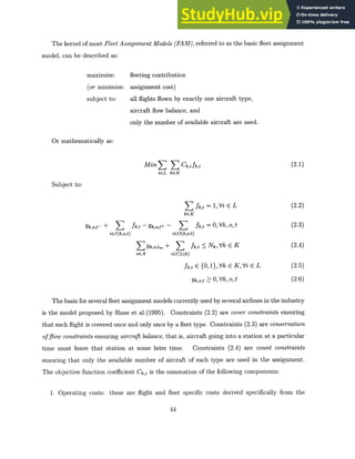
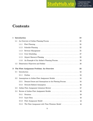
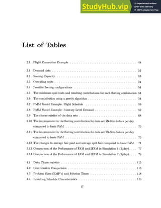
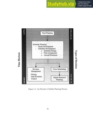
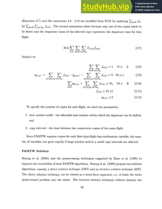
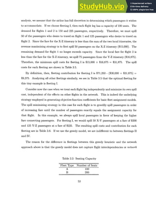
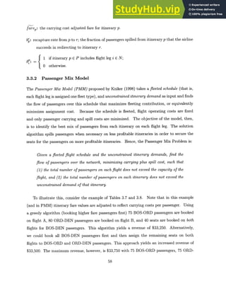
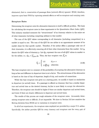
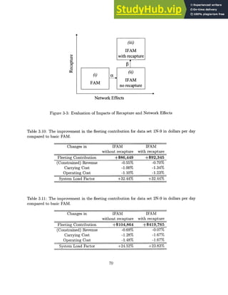
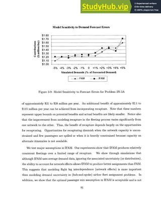
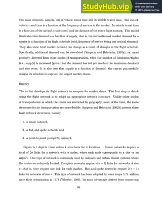
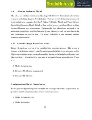
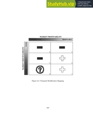
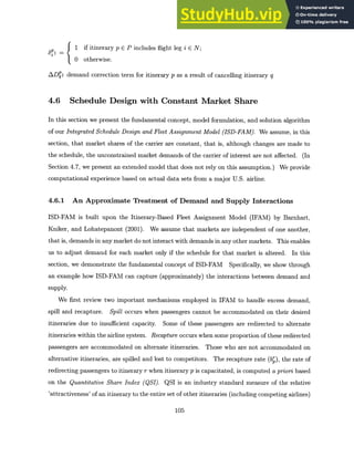
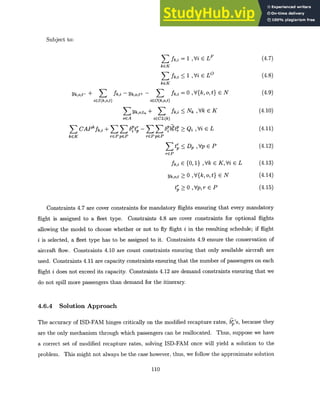
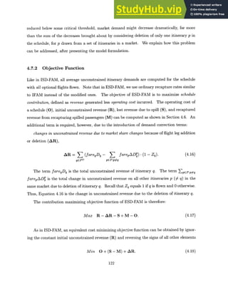
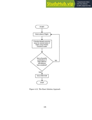
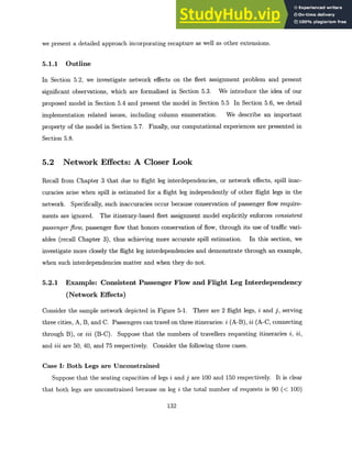
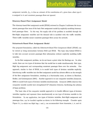
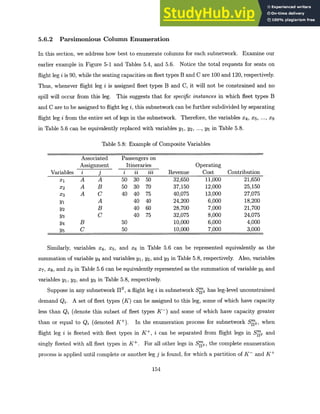
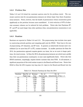
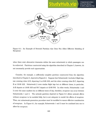
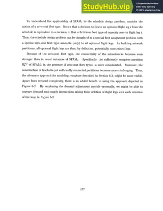
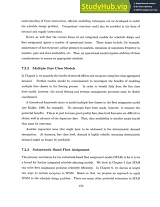
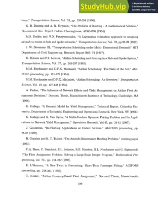
Step 1. Fare Allocation: From Itinerary to Flight Leg. In this step, because FAM
assumes flight leg independence, itinerary-based passenger fares must be allocated to
flight legs. For a direct itinerary, fare allocation is straightforward because there is only
one flight leg. For itineraries containing more than one flight leg, several "heuristic"
schemes are possible. Two allocation schemes widely used in the industry are (a) full
fare allocation;and (b) mileage-basedpro-ratedfare allocation. In the former, each leg
in the itinerary is assigned the full fare of the itinerary; while in the latter, each leg in
the itinerary is assigned a fraction of the total fare, proportional to the ratio of the leg's
mileage to total mileage in the itinerary.
Step 2. Spill Estimation. There are two major approaches to spill estimation once fares
have been allocated.
Deterministic: Given the fare allocation of Step 1, spill is determined for each
flight leg based on its capacity, independent of other flight legs. The most common
spill estimation process considers a flight leg i and the unconstrained demand (pas-
sengers by itinerary) for i. It begins by listing the passengers in order of decreasing
revenue contribution, and then offering seats to those on the list, in order, until all
passengers are processed or capacity is fully utilized. If the capacity is sufficient to
carry all passengers, no spill occurs and spill cost for leg i is zero. If, on the other
hand, demand exceeds capacity, lower ranked passengers are spilled and the total
revenue of these spilled passengers is the estimated spill cost for flight leg i.
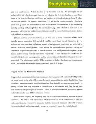
Probabilistic: The estimated spill cost of assigning fleet type k to leg i is com-
puted as the product of an average spill fare, SFk,i, and expected number of spilled
passengers,E[tk,i]. The expected number of spilled passengers, E[tk,i], is estimated
for flight leg i with assigned fleet type k, assuming that the flight leg level demand
distribution is Gaussian. The standard parameters for the Gaussian distribution
used in this context are: expected demand Qj, average number of passengers trav-
eling on flight leg i, and standard deviation K * Qi, where K is between 0.2 and
0.5. Alternatively, another popular estimate for the standard deviation is Z * ,
where Z is between 1.0 and 2.5. Details of this process can be found in Kniker
46

(1998).
In basic FAM models, spill costs cannot be captured exactly for two reasons:
1. Spill costs in FAM models are estimated independently for each flight leg and each possible
fleet assignment to that leg. It is, however, impossible to decide which passengers to spill
from a particular leg i unless the capacities assigned to other flight legs (such as those
contained in itineraries including i) are also known.
2. Even if the number of passengers of each itinerary to spill from a flight leg were known, it
would not be possible to assign accurately the spill costs to individual flights, as required
in the basic FAM model and guarantee that the solution to the FAM model would indeed
be optimal.
Clearly, the basic FAM spill estimation step above is inexact for it does not allow for network
interdependency. Kniker and Barnhart(1998) experiment with several fare allocation schemes
and show that different allocation schemes generate different fleet assignment decisions, different
contributions, and that no one scheme consistently outperforms the others.
FAM Solution
Hane et al.(1995) demonstrate solution techniques for this model using an airline network with
2600 flights and 11 fleet types. The techniques they employ include:
1. node consolidation: an algebraic substitution technique that results in significant reduc-
tions in problem size;
2. island construction: an exploitation of special problem structure that achieves further
reduction in problem size; and
3. specialized branching strategies and priorities: branching based on special ordered sets
(SOS)1 and selection of variables on which to branch based on a measure of variability of
the objective coefficients.
'The cover constraints, which are of the form Ek fk,i = 1, are referred to as Type 3 SOS constraints. An
efficient branching strategy is to divide the set of variables into two sets, where the sum of the variables in the
first (or second) set equals 1, and the sum of the variables in the other set equals 0. This can lead to a more
balanced partitioning of the feasible sets in the branch-and-bound tree. (Hane et al., 1995)
47

Table 2.1: Flight Connection Example
Departure Ready
Flight Origin Destination Time Time Demand
A BOS ORD 0800 1000 150
B ORD DEN 0955 1200 150
Their approach solves daily fleet assignment problems for a major U.S. airline in approxi-
mately 30 minutes on workstation class computers.
2.4.4 The Fleet Assignment with Time Windows Model
The motivation for the development of the fleet assignment with time windows model (FAMTW)
(Rexing et al. 2000) is that by providing time windows within which flights can depart, a more
cost effective fleeting and schedule might be obtained. That is , the output of FAMTW is both
a fleet assignment and selected departure times (within pre-specified time windows) for each
flight leg. FAMTW can lead to reductions in fleet assignment costs in two ways:
1. opportunities arise to assign a more appropriate aircraft type to a flight leg when flight
departures are re-timed because more aircraft connections are possible, and
2. aircraft can be more efficiently utilized given re-timings in the flight schedule and this can
result in a fewer number of aircraft needed to fly the schedule.
To illustrate the idea of time windows, consider Table 2.1 (Rexing et al. 2000). The demand
on both flights A and B is the same. Therefore, it may be appropriate to assign the same
aircraft to both flight legs. However, this is currently impossible because the ready time of
flight A is later than the departure time of flight B. By either allowing flight A to depart a little
earlier or flight B to depart a little later (or both), we can fly both flights with a single aircraft.
The variable definitions are the same as in FAM except f,,k,i is the binary variable that
takes on value 1 if copy n of flight i is covered by fleet type k and 0 otherwise and Nki is
the set of copies of flight i for fleet type k. Flight copies of a flight represent that same flight
at different departure times. The copy interval defines how far apart a copy is placed from
its preceding copy. At the extreme, copies are placed every minute. The objective function
48

(Equation 2.7) and the constraints 2.8 - 2.10 are modified from FAM by replacing EkEK fk,i
by ZkEK EnENki fn,k,i. The second summation arises because only one of the copies needs to
be flown and the departure times of the selected copy represents the departure time for that
flight.
(2.7)
Min E I Cn,k,ifn,k,i
iEL kGKnGNi
Subject to:
Vi E L (2.8)
fn,k,i = 1
kGK nENki
Yk,o,t- + fn,k,i - Yk,o,t+ - fn,k,i = 0
iEI(k,o,t) nENki iEO(k,o,t) nENki
E Yk,o,tn + fn,k,i < Nk
oGO iCCL(k) nENki
fn,k,i E {0, 1}
Yk,o,t >_ 0
Vk, o, t
Vk e K
(2-9)
(2.10)
(2.11)
(2.12)
To specify the number of copies for each flight, we need two parameters:
1. time window width-theallowable time window within which the departure can be shifted,
and
2. copy interval-thetime between two consecutive copies of the same flight.
Since FAMTW requires copies for each fleet-type-flight-leg-combination variable, the num-
ber of variables can grow rapidly if large window and/or a small copy intervals are selected.
FAMTW Solution
Rexing et al. (2000) uses the preprocessing techniques suggested by Hane et al. (1995) to
improve the tractability of their FAMTW algorithms. Rexing et al. (2000) propose two solution
algorithms, namely, a direct solution technique (DST) and an iterative solution technique (IST).
The direct solution technique can be viewed as a brute-force approach, i.e., it loads the entire
preprocessed problem into the solver. The iterative solution technique reduces memory size
49

requirements by exploiting the fact that only selected flight copies are in an optimal solution.
The difficulty is to identify which flight copies are necessary. The IST algorithm addresses
this difficulty by first solving the fleet assignment problem on a special network containing
only reduced-durationflight arcs, that is, flight arcs that begin at the latest possible times
and end at the earliest possible times. The resulting fleet assignment is used to partition the
flights by assigned fleet type. Then, for each fleet, feasibility of the assignment is checked using
original flight times and special arcs called backward arcs that identify infeasible assignments.
The flights associated with these infeasible assignments are the flights whose reduced- duration
flight arc are replaced by flight copies in the next iteration, the fleet assignment problem is
solved over this hybrid network. The process repeats until no infeasible assignments exist and
hence, an optimal assignment has been found.
2.5 Summary
In Section 2.2, we discuss several assumptions generally made in most fleet assignment mod-
els. Some assumptions are made to simplify the modeling process (for example, fare class
aggregation), while some are designed to simplify the operations (for example, day-of-week ag-
gregation). We next review the literature on the fleet assignment problem, showing that fleet
assignment is a well studied problem. There are, however, several aspects of the problem that
are modeled only approximately or entirely ignored, hence, room for improvement exists. A
detailed review of two basic fleet assignment models is presented. The basic fleet assignment
model by Hane, et al. (1985), in particular, will serve as a basis for development and discussion
throughout this dissertation.
50

Chapter 3
Network Effects and Recapture in
the Airline Fleet Assignment
Problem
3.1 Introduction
Recall from Section 2.2 that because a significant proportion of passengers travel on multi-leg
itineraries, flight legs in the network are interdependent. Specifically, in order to offer a service
to a passenger requesting a multi-leg itinerary, the airline must know that there are open "seats"
available on all flight legs contained in the itinerary. The influence of such interdependency
can be significant, because if ignored, it can lead to large errors in revenue estimation. We
refer to these phenomena as network effects.
Most basic fleet assignment models, however, ignore this interdependency and assume that
flight legs are independent. We collectively refer to the fleet assignment models that ignore
network effects as leg-basedfleet assignment models. In particular, in leg-based fleet assignment
models, estimates of revenue from assigning a fleet type to a flight leg are computed without
consideration of other flights and fleet assignments in the network.
Another aspect that is often modeled only approximately or completely ignored, is demand
recapture. Recapture occurs when passengers are carried on alternate itineraries because their
51

desired itineraries are capacitated. Leg-based fleet assignment models can at best approximate
this process because they do not model exact capacity of other flight legs. We show in this
chapter that incorporating flight leg interdependency and recapture in the fleeting process can
lead to better assignments.
3.1.1 Outline
In Section 3.2, we illustrate the importance of considering network effects in the fleeting process.
In Section 3.3, we review two relevant models: the Passenger Mix Model (PMM) and the
Itinerary-BasedFleet Assignment Model (IFAM). We describe the characteristics of our data
sets in Section 3.4. In Section 3.5, we present a case study performed on two full-scale data sets
(provided by a major U.S. airline) comparing the solution quality using a basic fleet assignment
model and our itinerary-based fleet assignment model. In Section 3.6,we present experiments
evaluating the sensitivity of our approach to its underlying demand and recapture assumptions.
3.2 Network Effects
To illustrate the effects of flight leg interdependencies (network effects) on spill and recapture,
consider the example described in Tables 3.1, 3.2and 3.3. Table 3.1 shows demand and fare
data in three markets, X-Y, Y-Z, and X-Z (connecting through Y). Table 3.2 shows the seating
capacity for each fleet type. Table 3.3 shows operating costs for each possible fleet to flight
assignment. Note that for simplicity, we ignore passenger related costs for the moment. Table
3.4 lists all possible fleeting combinations for this small example, along with their associated
operating costs.
Table 3.1: Demand data
Market Itinerary Number of Average
(Sequence of Flights) Passengers Fare
X-Y 1 75 $200
Y-Z 2 150 $225
X-Z 1-2 75 $300
The unconstrained revenue is 75($200) + 150($225) + 75($300) = $71,250. For the following
52

analysis, we assume that the airline has full discretion in determining which passengers it wishes
to accommodate. If we choose fleeting I, then each flight leg has a capacity of 100 seats. The
demand for flights 1 and 2 is 150 and 225 passengers, respectively. Therefore, we must spill
50 of the passengers who desire to travel on flight 1 and 125 passengers who desire to travel on
flight 2. Since the fare for the X-Z itinerary is less than the sum of the two local itineraries, the
revenue maximizing strategy is to first spill 50 passengers on the X-Z itinerary ($15,000). The
remaining demand for flight 1 no longer exceeds capacity. Since the local fare for flight 2 is
less than the fare for the X-Z itinerary, we spill 75 passengers from the Y-Z itinerary ($16,875).
Therefore, the minimum spill costs for fleeting I is $15,000 + $16,875 = $31,875. The spill
costs for each fleeting are shown in Table 3.5.
By definition, then, fleeting contribution for fleeting I is $71,250 - ($30,000 + $31,875) =
$9,375. Analyzing all other fleetings similarly, we see in Table 3.5 that the optimal fleeting for
this tiny example is fleeting I.
Consider now the case when we treat each flight leg independently and minimize its own spill
cost, independent of the effects on other flights in the network. This is indeed the underlying
strategy employed in generating objective function coefficients for basic fleet assignment models.
The spill minimizing strategy in this case for each flight is to greedily spill passengers in order
of increasing fare until the number of passengers exactly equals the assignment capacity for
that flight. In this example, we always spill local passengers in favor of keeping the higher
fare connecting passengers. For fleeting I, we would spill 50 X-Y passengers at a fare of $200
and 125 Y-Z passengers at a fare of $225. The resulting spill costs and contribution for each
fleeting are in Table 3.6. If we use the greedy model, we are indifferent to between fleetings II
and IV.
The reason for the difference in fleetings between this greedy heuristic and the network
approach above is that the greedy model does not capture flight interdependencies or network
Table 3.2: Seating Capacity
Fleet Type Number of Seats
A 100
B 200
53

Table 3.3: Operating costs
Fleet Type Flight 1 Flight 2
A $10,000 $20,000
B $20,000 $39,500
Table 3.4: Possible fleeting configurations
Fleeting Flight 1 Flight 2 Total Operating Cost
I A A $30,000
II A B $49,500
III B A $40,000
IV B B $59,500
Table 3.5: The minimum spill costs and resulting contributions for each fleeting combination
Fleeting Operating Costs Spilled Passengers Spill Costs Contribution
I $30,000 50 X-Y, 75 Y-Z $31,875 $9,375
II $49,500 25 X-Z, 25 X-Y $12,500 $9,250
III $40,000 125 Y-Z $28,125 $3,125
IV $59,500 25 Y-Z $5,625 $6,125
Table 3.6: The contribution using a greedy algorithm
Fleeting Operating Costs Spilled Passengers Spill Costs Contribution
I $30,000 50 X-Y, 125 Y-Z $38,125 $3,125
II $49,500 50 X-Z, 25 X-Y $15,625 $6,125
III $40,000 125 Y-Z $28,125 $3,125
IV $59,500 25 Y-Z $5,625 $6,125
54

effects. The best set of passengers to spill from one flight leg is a function of the demands
and assigned capacity on other flight legs. The myopic solution can be improved by taking a
network-wide view of the problem and spilling connecting passengers and accommodating local
passengers. Most basic fleet assignment models, however, ignore network effects and assume
flight leg independence, therefore, their solutions are often suboptimal.
In this small example, it is possible to enumerate possible fleeting combinations and compute
the minimum spill costs accordingly. However, with a network of hundreds or thousands of
flight legs, enumeration is computationally expensive, if not impossible. Thus, we describe a
new modeling and algorithmic approach for fleet assignment that models spill and recapture as
a function of assigned capacity across an entire airline network, and not just a single flight leg.
3.3 Review of Passenger Mix and Itinerary-Based Fleet Assign-
ment Models
3.3.1 Terminology and Notation
Terminology
To facilitate the description of the passenger mix and fleet assignment models, we define the
following terms. A flight leg is a non-stop trip of an aircraft from an origin airport to a
destination airport (one take-off and one landing). A market is an ordered origin-destination
airport pair, in which passengers wish to fly. Boston Logan International (BOS) - Chicago
O'Hare (ORD), for example, is a distinct market from ORD-BOS, which is an opposite market.
An itinerary in a particular market consists of a specific sequence of scheduled flight legs, in
which the first leg originates from the origin airport at a particular time and the final leg
terminates at the final destination airport at a later time. We model a round-trip itinerary
as two distinct trips in two opposite markets. A Boston-Chicago round-trip is represented as a
passenger in the BOS-ORD market and a passenger in the ORD-BOS market. A market may
have numerous itineraries.The itinerary comprised of flight 789 from BOS to ORD and flight
276 from ORD to Los Angeles International (LAX) is distinct from the itinerary comprised
of flight 792 from BOS to ORD and flight 275 from ORD to LAX, of which both are in the
55

BOS-LAX market, but scheduled at different times.
Often times the modifier unconstrained is used to denote that the quantity of interest is
measured or computed without taking into account any capacity restrictions. For example,
unconstraineddemand of an airline in a market is the total (share of) demand (or request for
air travel) as experienced by the airline of interest in a market regardless of flights or
seats offered. This should be distinguished from constraineddemand, which is the total demand
accommodated by the airline, subject to available aircraft capacity. Recall, also, our convention
that unconstrained demand always refers to the (share of) demand of the airline of interest,
not that of the entire market, unless explicitly noted otherwise. Similarly, unconstrained
revenue is the maximum revenue attainable by the airline independent of capacity offered;
while constrainedrevenue is the achievable revenue subject to capacity constraints.
We assume our schedule is daily, that is, the schedule repeats itself every day. Thus,
the end of the day is connected to the beginning of the day by a wrap-around arc. The
extension to a weekly schedule is straightforward. Airlines, however, prefer solving for the
daily schedule because they can maintain fleeting consistency throughout the week and thus
minimize operational complications.
In order to count the number of aircraft in the network, we take a snapshot of the network
at some point in time and count the number of aircraft both in the air and on the ground at
stations. The exact time that we take the snapshot, defined as the count time, does not matter
because conservation of aircraft flow is required throughout the network.
Notation
Sets
P: the set of itineraries in a market indexed by p or r.
A: the set of airports, or stations, indexed by o.
K: the set of fleet types indexed by k.
T: the sorted set of all event (departure or availability) times at all airports, indexed by tj. The
56

event at time t3 occurs before the event at time tj+1. Suppose IT = m; therefore ti is
the time associated with the first event after the count time and tm is the time associated
with the last event before the next count time.
N: the set of nodes in the timeline network indexed by {k, o, t3 }.
I(k, o, t): the set of inbound flight legs to node {k, o, t}.
O(k, o, t): the set of outbound flight legs from node {k, o, t}.
Decision Variables
tp: the number of passengers requesting itinerary p but redirected by the model to itinerary r.
=k,i: 1 if flight leg i E N is assigned to fleet type k E K;
0 otherwise.
yk,o,t: the number of fleet type k aircraft that are on the ground at airport o C A immediately
before time ti E T. If ti and t2 are the times associated with adjacent events, then
Yk,o,t+ = Yk,o,t-
Parameters/Data
CAP: the number of seats available on flight leg i (assuming fleeted schedule).
SEATSk: the number of seats available on aircraft of fleet type k.
Nk: the number of aircraft in fleet type k, Vk C K.
D,: the unconstrained demand for itinerary p, i.e., the number of passengers requesting itinerary
p-
farep: the fare for itinerary p.
57

farep: the carrying cost adjusted fare for itinerary p.
b : recapture rate from p to r; the fraction of passengers spilled from itinerary p that the airline
succeeds in redirecting to itinerary r.
1 if itinerary p E P includes flight leg i E N;
0 otherwise.
3.3.2 Passenger Mix Model
The PassengerMix Model (PMM) proposed by Kniker (1998) takes a fleeted schedule (that is,
each flight leg is assigned one fleet type), and unconstraineditinerarydemand as input and finds
the flow of passengers over this schedule that maximizes fleeting contribution, or equivalently
minimizes assignment cost. Because the schedule is fleeted, flight operating costs are fixed
and only passenger carrying and spill costs are minimized. The objective of the model, then,
is to identify the best mix of passengers from each itinerary on each flight leg. The solution
algorithm spills passengers when necessary on less profitable itineraries in order to secure the
seats for the passengers on more profitable itineraries. Hence, the Passenger Mix Problem is:
Given a fleeted flight schedule and the unconstrained itinerary demands, find the
flow of passengers over the network, minimizing carryingplus spill cost, such that
(1) the total number of passengers on each flight does not exceed the capacity of the
flight, and (2) the total number of passengers on each itinerary does not exceed the
unconstraineddemand of that itinerary.
To illustrate this, consider the example of Tables 3.7 and 3.8. Note that in this example
(and in PMM) itinerary fare values are adjusted to reflect carrying costs per passenger. Using
a greedy algorithm (booking higher fare passengers first) 75 BOS-ORD passengers are booked
on flight A, 80 ORD-DEN passengers are booked on flight B, and 40 seats are booked on both
flights for BOS-DEN passengers. This algorithm yields a revenue of $33,250. Alternatively,
we could book all BOS-DEN passengers first and then assign the remaining seats on both
flights to BOS-ORD and ORD-DEN passengers. This approach yields an increased revenue of
$33,500. The maximum revenue, however, is $33,750 with 75 BOS-ORD passengers, 75 ORD-
58

Table 3.7: PMM Model Example: Flight Schedule
Flight Origin Destination Departure Arrival Capacity
A BOS ORD 9:45 am 11:23 am 120
B ORD DEN 12:00 pm 1:31 pm 120
Table 3.8: PMM Model Example: Itinerary Level Demand
Itinerary Origin Destination Departure Arrival Demand Adjusted Fare
A BOS ORD 9:45 am 11:23 am 75 150
B ORD DEN 12:00 pm 1:31 pm 80 150
C BOS DEN 9:45 am 1:31 pm 50 250
DEN passengers, and 45 BOS-DEN passengers assigned. From this tiny example, we can see
that the mix of passengers on flights can affect revenues substantially.
To formulate the passenger mix problem, we denote fare, as the adjusted fare for itinerary
r, i.e., fare less carrying cost for itinerary r. We let 'P represent the number of passengers
spilled from itinerary p and redirected to itinerary r. In this formulation, we explicitly model
recapture phenomenon using recapturerates,bp for each r E R, and p E P, denoting the fraction
of passengers spilled from itinerary p whom the airline succeeds in redirecting to itinerary r.
The product of t; and bpr is therefore the number of passengers recaptured from itinerary p
onto itinerary r. We denote tH as spill from itinerary p to a null itinerary and assign its
associated recapture rate, b , a value of 1.0. Passengers spilled from itinerary p onto a null
itinerary are not recaptured on any other itinerary of the airline and are lost to the airline.
The mathematical formulation for PMM is:
Min ( farep - b farer)t
pGP rGP
(3.1)
59

Subject to:
ZZ Zit;-Irb tP>Qi-CAP ,ViEL (3.2)
pEP rEP rEPpEP
St DP ,Vp EP (3.3)
rEP
t; > 0 ,Vp,r E P (3.4)
Notice that this formulation utilizes a special set of variables (keypath variables tr), first
proposed by Barnhart et al.(1995), to enhance model solution. Note also that the objective
function minimizes spill plus carrying costs, or equivalently, assignment cost. Constraints (3.2)
are the capacity constraints. For leg i, the term ErEP ZEPP 6ptr - pEP 6p3t can be viewed
as the number of passengers who are spilled from their desired itinerary p. For leg i, the term
ZrEP pEP - EPtp 6PpbtZp is the number of passengers who are recaptured by the airline.
(Note that we assume b, = 1.) CAP is the capacity of the aircraft assigned to leg i, and Qi is
the unconstrained demand on flight leg i, which can be written mathematically as,
Qi= Z
E Dp. (3.5)
pEP
Constraints (3.3) are the demand constraints that restrict the total number of passengers spilled
from itinerary p to the unconstrained demand for itinerary p. tp is must be greater than zero
but need not be integer because we model the problem based on average demand data, which
can be fractional.
An Itinerary-Based Spill Model
PMM, an itinerary-based spill model, differs from the leg-based spill models widely used in the
industry to compute spill costs for basic FAM models. To understand these differences, let t,(i)
represent spill from itinerary p to itinerary r, on flight leg i, and farep(i) be the representative
adjusted fare of itinerary p, allocated to flight leg i. Assume that EiEP farep(i)8p = farep
and that there is no recapture. Then, we can rewrite (3.1) - (3.4) as:
60

Min E farep(i) * 6Ptp(i) (3.6)
iGL pGP rGP
Subject to:
6 it (i) Qi - CAP Vi (E L (3.7)
rC~pCP
rGPPE P
E 6Pt (i) < DpVpEPViEL (3.8)
rEP
t=(i) _ t O
= Vp,rEPVi Ep (3.9)
tp(i) > 0Vp,rEPViEL (3.10)
This model is equivalent to PMM for cases with bp = 0 and EiCL farep()8 farep. By
relaxing equations (3.9), we obtain a leg-based spill model that optimizes t (i) independently
of tP(j), for i, j contained in p. This is exactly the approach for estimating spill cost in the
basic FAM model described in section 2.4.3.
Hence, PMM overcomes some of the problems encountered in estimating spill costs in basic
FAM by:
1. forcing all spills from the same itinerary p to be equal for all flight legs contained in p and
2. eliminating the unnecessary step of allocating fare among flight legs i contained in p.
PMM also models recapture, an impossibility in leg-based spill models because spill is
modeled only approximately.
PMM Solution
To solve PMM, the second set of constraints is relaxed initially. The rationale is that there
can be many of these constraints, one for each itinerary, and the constraints are not likely
to be binding in optimal solutions. To understand why, observe that the objective function
coefficients are typically positive. Even though most of the time the fare of itinerary r is higher
than that of itinerary p, the actual fare collected is scaled down by the recapture rate, which
61

can be a small number. Notice also that if r is the same as p, i.e., the passengers are not
redirected to any other itineraries, then the net effect on the objective function is zero. Since
most of the objective function coefficients are positive, an optimal solution reduces t' values
as much as possible. As a result, constraints (3.3) will not be binding typically. Similarly,
since most tr values are zero or close to zero, we can further reduce the size of the problem by
initially omitting all tr except those for null itineraries, t-. The rationale is that most of the
passengers will be carried on their desired itineraries; only in cases where capacities are limited
will spill and recapture occur.
Column and row generation techniques are then used to solve a restricted PMM, which
initially ignores constraints (3.3) and all t; variables except those for null itineraries, t . In
column and row generation techniques, subsets of variables and constraints are neglected to
create a restricted master problem. After solving the restricted master problem, pricing and
separationsubproblems are solved to identify columns that could potentially improve the so-
lution, and to identify violated constraints, respectively. These columns and constraints are
added to the restricted master problem and the process is repeated until no columns or rows are
generated. The solution approach for PMM is detailed in Kniker, Barnhart, and Lohatepanont
(2001) and results are presented using data from a large U.S. airline.
Upper Bound on Achievable Revenue
Suppose that unconstrained itinerary demands are known a priori with certainty, PMM provides
an upper bound on the achievable revenue because it assumes that the airline has full discretion
to redirect passengers to alternate itineraries when their desired itineraries are capacitated. In
reality, airlines have only estimates of demands due to uncertainty, and they do not have
full discretion over passengers' itineraries. Thus, in most circumstances, the actual revenue
achieved is smaller than PMM's estimated revenue.
In subsequent chapters, we frequently solve PMM to estimate achievable revenues of fleeted
schedules. We refer to such estimates as PMM revenues (or PMM contributions if costs are
subtracted from the revenues) to emphasize that they represent maximum achievable revenues
(or contributions), and not necessarily average or expected revenues (or contributions).
62

3.3.3 Itinerary-Based Fleet Assignment Model
The motivation for the Itinerary-BasedFleet Assignment Model (IFAM) is that FAM does not
accurately capture revenue because it ignores interactions between flight leg and demands. As
stated earlier, FAM requires as input the revenue for each fleet-type- flight-leg combination
(or equivalently the spill cost for each fleet-type-flight-leg combination). This is impossible to
compute exactly, however, until a fleeting is known. In IFAM, the dependence of these decisions
is modeled and operating costs and revenues can be computed much more accurately since the
fleet assignment and passenger mix problems are solved simultaneously.
Enhancing the basic fleet assignment model has been of interest to the airline industry and
researchers. Farkas (1995), and Jacobs, Smith and Johnson (1999), and Rexing, et al. (2000)
develop enhanced fleet assignment models that are able to capture several interesting aspects
of the problem not captured by FAM.
Farkas (1995) develops an itinerary-based fleet assignment model that combines the basic
fleet assignment model with a passenger mix model ignoring recapture. He presents two different
procedures for solving the model. The first procedure, a column generation approach, requires
the repeated solution of the basic fleet assignment model because each decision variable in
his model is a complete fleeting. To date, this approach is computationally impractical for
problems of the size encountered in the industry. Farkas also suggests a second, heuristic
approach that partitions the flight legs into sub-networks where network effects of multi-leg
itineraries are present.
Erdmann et al. (1997) present a sequential approach in which a fleet assignment model is
solved and then, given the resulting fleeting, a passenger mix problem is solved. They propose
various solution approaches, including Lagrangian relaxation.
Jacobs, Smith and Johnson (1999) present a different approach to the origin & destination
fleet assignment problem. In their implementation, a series of fleet assignment model relax-
ations and the combined fleet assignment and passenger flow problem are solved iteratively.
Once pre-specified criteria are met, the model is solved for the optimal integer solution.
Other improvements or extensions to basic FAM include, for example, Soumis, Ferland, and
Rousseau (1980), Ioachim et al (1999), Jarrah and Strehler (2000), and Rexing et al. (2000).
63

Formulation
Min >3 Ck, fki + > 3 (farep - b fare,)t (3.11)
iGL kGK pGPrGP
Subject to:
> f,i = 1 ,Vi E L (3.12)
kcK
Yk,o,t- + > fk,i - Yk,o,t+ -- > fk,i = 0 ,Vk, o, t (3.13)
E Yk,o,tm + > fk,i Nk ,Vk E K (3.14)
o-A iCCL(k)
> SEATSkfk,i + E6|tp- E36PbPtP > Qi ,Vi CL (3.15)
kGK rEPpGP rEPpEP
> tr, D,,VpCP (3.16)
rEP
fk,i E {0, 1} ,Vk E K,Vi E L (3.17)
Yk,o,t 0 ,Vk, o, t (3-18)
t; > 0 ,Vp,r c P (3.19)
IFAM integrates basic FAM and PMM. In IFAM, spill and recapture, and their associ-
ated costs, are decisions of the model. These decisions are constrained by other decisions,
namely the capacity assigned to the network. In this way, IFAM captures the network-wide
interdependencies of capacity and revenue, thus improving on basic FAM.
The objective of IFAM is to minimize assignment cost. In IFAM, the variable definitions
are the same as those in basic FAM and PMM except that CAP is now replaced by SEATSK,
denoting the capacity of fleet type k. The first three sets of constraints (equations (3.12) to
(3.14)) are constraints of basic FAM and the next two sets of constraints (equations (3.15) and
(3.16)) are the constraints of PMM. Note however, that there is a change in one of the terms
in the capacity constraints (3.15). Specifically, the first term on the left has been moved from
the right-hand-side because now, the capacity of the flight is also a variable.
64

Generalizing FAM
The IFAM formulation given in (3.11) - (3.19) can be seen as an "enhanced" or generalized basic
fleet assignment model including carrying costs, recapture, and passenger flow conservation
(network effects). To illustrate, consider the IFAM case where EiCL farep(>P = farep for all
p E P, carrying cost equals zero, and b= 0 for all p, r E P. Then, IFAM can be equivalently
rewritten as:
Min S ck,ifk,i + 55 3 farep(i)6ot(i)
iEL kEK iELpEPrEP
(3.20)
Subject to:
E fk,i
kcK
Yk,o,t- + k i - Yk,o,t+ - k,i
Y Yk,o,tm + fk,i
oGA iECL(k)
S SEATSk fk,i + X75 Ptp(i)
kEK p PrEP
56tr(i)
rEP
ti ()
t
= 1 , Vi E L
= 0 ,Vkot
* Nk ,Vk c K
* Qi ,Vi E L
D, ,EVp P,Vi E L
- t = 0 ,Vp,r E P, Vi E L
fk,i E {0, 1} ,Vk E K, Vi E L
k,o,t > 0 ,Vk, 0, t
r(i) >0 ,Vp,r E P, Vi E L
If constraints 3.26 are eliminated, the optimal spill decisions can be determined using the
greedy spill estimation procedure described for basic FAM (Chapter 2). This implies that
constraints (3.24), (3.25) and (3.29) can be eliminated and instead captured directly through
spill cost coefficients in the objective function. Hence, the optimal solutions to basic FAM are
the same as those for (3.20) - (3.29) with no carrying costs or recapture, and equations (3.26)
65
(3.21)
(3.22)
(3.23)
(3.24)
(3.25)
(3.26)
(3.27)
(3.28)
(3.29)

eliminated, that is, conservation of passenger flows (network effects) ignored. IFAM, therefore,
improves upon basic FAM by capturing network effects as well as recapture and carrying costs.
Recapture Rates
Determining the recapture rates for alternative itineraries is itself a difficult problem. The basis
for calculating the recapture rates in these experiments is the QuantitativeShare Index (QSI).
This industry standard measures the "attractiveness" of an itinerary relative to the entire set
of other itineraries (including competing airlines) in that market.
The sum of the QSI values corresponding to all itineraries (including competitors) in a
market is equal to one. The sum of the QSI for one airline is an approximate measure of its
market share for that specific market. Therefore, if the airline offers a passenger only one of
their itineraries, it is effectively removing all of their other itineraries from this market. Let qp
denote the QSI value of itinerary p. Let Qm represent the sum of all QSI values in market m
for the airline, i.e., Qm = Zpem qp. Then, the base recapture rate, b is:
_r 1.0 if p=r
fi
=if r(3.30)
otherwise.
The base recapture rate is a measure of the probability of accepting the alternative itinerary as
long as fare and difference in departure time is not a factor. The attractiveness of the alternative
is based on the time of day of departure, length of trip, and number of connections.
While this base recapture rate gives us a starting point, we modify it based on similarities
in departure (or arrival) times. If a passenger is offered an itinerary that has a similar depar-
ture and arrival time as the desired itinerary, he/she is more likely to accept the alternative.
Therefore, the recapture rate should be higher if there are similar departure and arrival times,
and lower if there are drastic differences in departure and arrival times.
The results of this process are rough estimates of the recapture rates. Accurately deter-
mining recapture rates is difficult, if not impossible. We show in Section 3.6 how sensitive the
fleeting decisions from IFAM are to variations in recapture rates.
In all of our experiments, the recapture rates employed are provided by a major U.S. airline.
Specifically, the airline provides QSI for every itinerary and recapture rate for every pair of
66

Step 1 Step 2
Build Restricted -+ Coefficient Reduction
Master Problem Preprocessing
Step3 Yes
Solve RMP LP
Step 4 Were
Fviolated Con. G.WeeStep 7
any rows, No Branch &
columns or Bound
Step5 cuts added
Column Generation
Step 6 DONE
Spill Part. Cut Gen. Solve IFAM
LP Relaxation:
Figure 3-1: The direct solution approach for the combined fleet assignment and passenger mix
model
itineraries is computed according to Equation 3.30.
Overview of the Solution Approach
The overall IFAM solution approach is depicted in Figure 3-1. We construct a restricted master
problem (RMP) excluding constraints (3.16) and spill variables that do not correspond to null
itineraries. Next we apply a pre-processing step involving coefficient reduction, to tighten
the IFAM LP relaxation. Details of this step will be covered later in this section. Then
the LP relaxation of the restricted master problem is solved using column and row generation.
Negative reduced cost columns corresponding to spill variables, violated constraints (3.16) and
cuts (Step 6) are added to the RMP and the RMP is resolved until the IFAM LP relaxation is
solved. Given the IFAM LP solution, branch-and-bound is invoked to find an integer solution.
An optimal IFAM solution could be determined using a branch-and-price-and-cut algorithm
in which columns and constraints are generated within the branch-and-bound tree. Because
column generation at nodes within the branch-and-bound tree is non-trivial to implement using
available optimization software, we instead employ a heuristic IP solution approach in which
67

branch-and-bound allows column generation only at the root node.
Upper Bound on Contribution
We refer to the contributions computed from optimal IFAM solutions as IFAM contributions.
Similar to PMM contributions, IFAM contributions represent the maximum achievable contri-
bution of a given schedule because embedded in IFAM is PMM, which assumes ideal operations.
We present, at the end of this Chapter, a series of sensitivity analyses to evaluate some of the
assumptions in PMM and IFAM.
3.4 Data
Our models are tested and calibrated using data from a major U.S. airline. Table 3.9 describes
the characteristics of our data sets.
Table 3.9: The characteristics of the data sets
Data Set Number of Number of Number of Number of
Fleets Flight Legs Markets Itineraries
1N-3A 3 157 6,352 9,845
2N-3A 3 173 7,034 11,877
1N-9 9 2,044 20,928 76,641
2N-9 9 1,888 21,062 75,484
Data sets 1N-9 and 2N-9 are two full size data sets with 9 fleet types, whereas data sets 1N-
3A and 2N-3A are two smaller data sets extracted from the corresponding full size schedules.
1N-3A and 2N-3A, each includes 3 fleet types. Data set 1N-9, a schedule in the winter season
has less demand than data set 2N-9, a schedule in the summer season.
Our estimates of IFAM's benefits are based on contributions from the two full size data sets.
The two small data sets are used only to test sensitivity of the models to a number of factors.
3.5 Analysis of IFAM Contribution
In this section, we measure the improvement of the IFAM solution over that of basic FAM. The
analysis is prepared for results from runs on two full size networks, i.e., 1N-9 and 2N-9. We
68

or
FAM
Fleeting Decision
PMM:
Minimized Spill Operating Cost
and
Carrying Costs
Fleeting Contribution
Figure 3-2: Methodology
attempt to explain the improvement in contribution attributable to: (a) network effects; and
(b) recapture.
To determine the independent impacts of network effects and recapture on fleeting contri-
bution, we begin by solving basic FAM (Figure 3-3, Block i) using a mileage-based pro-rated
fare allocation scheme (an industry standard approach, described in Chapter 2), and ignoring
recapture. In order to quantify the impact of network effects, independent of recapture, we
solve IFAM with no recapture (Figure 3-3, Block ii). To consider recapture we solve IFAM
with recapture (Figure 3-3, Block iii). For each block, we apply the procedure in Figure 3-2
to obtain its associated fleeting contribution. In Figure 3-3, a represents the improvement in
fleeting contribution derived from capturing network effects and 3 represents the improvement
in fleeting contribution derived from incorporating recapture into the fleeting process.
3.5.1 Results and Analysis
Tables 3.10 and 3.11 report the fleeting contributions associated with FAM (Block i), IFAM
without recapture (Block ii), and IFAM (Block iii) with recapture.
The improvement (a) in contribution from including network effects in the fleeting process
69

(iii)
IFAM
with recapture
(i) (ii
FAM j IFAM
no recapture
Network Effects
Figure 3-3: Evaluation of Impacts of Recapture and Network Effects
Table 3.10: The improvement in the fleeting contribution for
compared to basic FAM.
data set 1N-9 in dollars per day
Changes in IFAM IFAM
without recapture with recapture
Fleeting Contribution +$86,449 +$92,345
(Constrained) Revenue -0.55% -0.70%
Carrying Cost -1.00% -1.34%
Operating Cost -1.10% -1.23%
System Load Factor +32.44% +32.44%
Table 3.11: The improvement in the fleeting contribution for
compared to basic FAM.
data set 2N-9 in dollars per day
Changes in IFAM IFAM
without recapture with recapture
Fleeting Contribution +$104,864 +$419,765
(Constrained) Revenue -0.69% -0.07%
Carrying Cost -1.28% -1.67%
Operating Cost -1.48% -1.67%
System Load Factor +24.52% +23.83%
70
0
A

ranges from $86,449 per day in problem 1N-9 to $104,864 per day in problem 2N-9, or, assuming
schedule and demand are the same for the entire 365-day year, from $31.5 million to $38.3
million per year. The additional improvement (/3) achieved by including recapture in the
fleeting process ranges from $5,896 per day in problem 1N-9 to $314,901 per day in problem
2N-9, or $2.1 million to $115.0 million per year. The total improvement in IFAM's fleeting
contribution compared to FAM, thus ranges from $33.7 million for 1N-9 to $153.2 million per
year for 2N-9. Note that the experiments are performed in a controlled and limited environment
assuming full airline discretion to accommodate passengers (an assumption in PMM). In other
words, these experiments represent best-case-scenario analysis of IFAM contributions. Thus,
these figures represent upper bounds on the achievable improvements, and do not necessarily
represent the actual or expected improvements.
Notice that the impact of modeling recapture in problem 2N-9 is significantly larger than
that in problem 1N-9. This is partly because the 2N-9 network is more congested due to higher
traffic level. (Recall that problem 2N-9 is drawn from a summer season.) Once the network
become more capacitated, within reasonable range, spill and recapture activities occur more
intensely. Opportunities for recapturing passengers arise. Thus, explicitly modeling recapture
in the fleeting process yields significant benefits. The benefit of this increased opportunity
for recapturing passengers will taper off when the network become significantly congested,
however, because there will be fewer empty seats elsewhere in the network to re-accommodate
the demand.
In analyzing these differences, we also observe that the operating cost is higher when the
schedule is fleeted using FAM. This implies that in FAM, the demand for a given flight leg
Table 3.12: The changes in average fare paid and average spill fare compared to basic FAM.
Changes in
Average Fare Paid Average Spill Fare
Problem 1N-9
IFAM without Recapture +0.08% -3.34%
IFAM with Recapture +0.12% -4.49%
Problem 2N-9
IFAM without Recapture +0.33% -5.94%
IFAM with Recapture +1.28% -14.62%
71

is overestimated and hence, too much capacity is assigned. This result is consistent with
our observations that in FAM, network effects cannot be captured and passengers on multi-leg
itineraries can be effectively spilled from one leg but not the others. The system load factor,
that is, the ratio of the total number of passengers carried to the total number of seats supplied,
is reported in Tables 3.10 and 3.11 for the FAM and IFAM solutions. By modeling network
effects more accurately, IFAM clearly is better able to match passenger loads with capacity.
Next we observe in problem 2N-9 that IFAM with recapture compared to IFAM without
recapture produces a fleet assignment generating more revenue and carrying fewer passengers
(note that carrying cost per passenger is constant across all aircraft types). The average fare
paid by passengers captured by the airline and the average fare of spilled passengers lost to the
airline, reported in Table 3.12, is evidence that IFAM with recapture is better able to make
fleeting decisions that allow high revenue passengers to be carried and low revenue passengers
to be spilled.
3.6 IFAM Sensitivity
In this section, we address several key assumptions built into IFAM, namely,
1. recapture rates,
2. deterministic demand, and
3. optimal passenger mix.
We show through empirical testing that IFAM needs only rough estimates of recapture rates.
The final contributions resulting from different fleeting decisions using varying recapture rates
vary within a small range and IFAM consistently outperforms FAM for a range of recapture
rates. As described in Chapter 2, the spill cost estimation in basic FAM recognizes certain
stochastic elements in demand. In this section, we show through simulations that although
IFAM does not consider demand uncertainty, its ability to model network effects and recap-
ture allows it to outperform FAM. Next, we evaluate the sensitivity of our approach to the
assumption that an optimal passenger mix is always achieved. We show through simulations
that although IFAM assumes that the airline has full control of passenger allocation and can
72

pb IFAM
Fleeting Decision
PMM:
Minimized Spill Operating Cost
tand ortin
Carrying Costs
E Fleeting Contribution
Figure 3-4: Methodology for Testing Model Senstitivity to Recapture Rate
thus derive an optimal passenger mix, IFAM continues to perform well in a more realistic, less
controlled environment.
In addition, because all fleet assignment models require forecast demand as input, we test
the sensitivity of both FAM and IFAM to demand forecast errors. Our experiment suggests
that, as expected, both FAM and IFAM are sensitive to such errors.
3.6.1 Sensitivity of Fleeting Decisions to Recapture Rates
One of the most difficult parameters to estimate in IFAM are recapture rates because they are
unobservable in reality. We show in this section, however, that we do not need highly accurate
estimates of recapture because, as our experiments show, the benefit of incorporating recap-
ture into the fleeting decision process outweights any errors that might result from inaccurate
recapture rates.
In this exercise, we assume that the actual recapture rate from itineraries p to r, is b and
the recapture rate from itineraries p to r that is used in IFAM model is bp. A fleeting decision
is derived from IFAM using bp as input. This fleeting is then used to estimate contribution
using b as input into the PMM model. Figure 3-4 depicts this process. Sensitivity analysis is
73

Recapture Rate Sensitivity
8,000
E - 7,000
. . 6,000 *
- 4 -
r 5,000
E 4,000
3,000
C 2,000
5 1,000
0
0.5 0.6 0.7 0.8 0.9 1 1.1 1.2 1.3 1.4 1.5
Recapture Rate Multiplier (5)
+ Sensitivity of IFAM
-. - Improvement gained from network effects alone
-- Improvement gained from network effects and recapture
Figure 3-5: Recapture Rate Sensitivity for 1N-3A Data Set
performed based on differing by's, which are computed by multiplying scaling factors, 6's, and
the actual recapture rate, b", that is,
br = br. (3.31)
To form the basis for the comparison, we solve FAM and computed the estimated contri-
bution using the PMM model with actual recapture rates, br. We perform this experiment on
two small data sets, namely, 1N-3A and 2N-3A. The allowable integrality gaps for IFAM are
set at $1,000 daily for both problems. The results are graphed and shown in Figures 3-5 and
3-6. We vary 6 from 0.5 to 1.5 at a 0.1 step. 6's are plotted on the horizontal axis. Note that
6 equals 1.0 means that we input the correct set of recapture rates into our IFAM model. The
solid lines in Figures 3-5 and 3-6 show the improvement gained from considering network effects
and recapture in IFAM when average daily demand and the correct recapture rates are input.
The dashed lines show the improvement gained from considering only network effects. Thus,
the distance between the solid and dashed lines measures the benefit of recapture. Each dia-
mond represents the improvement of IFAM over FAM when b rates are used in IFAM. Thus,
the distance from the solid line to each diamond measures the error from underestimating or
74

Recapture Rate Sensitivity
60,000
50,000 ,
40,000-
E 20,000
0. 10,000
0
0.5 0.6 0.7 0.8 0.9 1 1.1 1.2 1.3 1.4 1.5
Recapture Rate Multiplier (6)
+ SensithAty of IFAM
- - Improvement gained from network effects alone
Improvement gained from network effects and recapture
Figure 3-6: Recapture Rate Sensitivity for 2N-3A Data Set
overestimating the actual recapture rates by a factor of 6.
In Figure 3-5, the daily improvement of IFAM over FAM is approximately $7,500 with
recapture and $5,600 without recapture. Thus, the daily benefit of considering recapture is
$1,900. When very low recapture rates are used in IFAM, there are essentially no benefits to
considering recapture in the fleeting process. When recapture rates are increased, the benefit
increases. IFAM does not, however, appear to be particularly sensitive to the rates of recapture,
over a small range of values. As seen in Figure 3-5, the benefits of recapture remain relatively
constant over a range of 6, then jump to another level and, again, remain relatively constant. In
Figure 3-6, the daily improvement of IFAM over FAM is approximately $47,500 with recapture
and $30,000 without recapture. The daily benefit of considering recapture is $17,500. In this
data set, we observe again that IFAM's improvement relative to FAM increases as we increase
recapture rates. The improvement reaches a certain level and remains relatively constant
throughout. Note, however, that when 6 equals 1.5 in Figure 3-6, a significant deterioration is
observed. This is possible because the overestimated recapture rates are used when IFAM tries
to optimize the fleeting, thus, IFAM would assign smaller aircraft to flight legs in an attempt
to save operating costs anticipating that the spilled passengers are recaptured on other flight
legs. When actual recapture is used to estimate contribution, however, the expected recaptured
75

Average FAM
Unconstrained or
Demand IFAM
Fleeting Decision
Passenger
Allocation Operating Cost
Simulation
Fleeting Contribution
Figure 3-7: Methodology for Simulation 1 (Measuring the Performance of FAM and IFAM
under simulated environment)
demand does not materialize, resulting in decreased profitability.
Although we perform these experiments on two small problems, the problems mimic closely
the nature of larger problems. The results from this experiment suggest that the fleeting
decision of IFAM is not particularly sensitive to recapture rates, for a reasonable range of
rates.
3.6.2 Demand Uncertainty
In this section, we measure the performance of IFAM compared to FAM in a simulated environ-
ment where realizations of forecasted demand vary by day of week. It is possible theoretically
to solve IFAM for every day in a week and have different fleetings for the same flight on differ-
ent days. This is, however, often impractical from an operational standpoint. Thus, airlines
typically solve the fleet assignment model based on average demand data.
In basic FAM, this average demand data is computed at the leg level and is assumed to have
a normal distribution with mean equal to average demand and standard deviation as described
in Chapter 2. Based on this assumption, basic FAM estimates the spill cost of assigning fleet
76

type k to flight leg i independently of other legs in the network using a spill model. In IFAM,
this average demand data is computed at the itinerary level and is used as a representative
realization of the demand. Then, the model is solved, taking into account network effects and
recapture.
In this section, we compare how the fleeting decisions from FAM and IFAM compare under
a simulated environment. Figure 3-7 depicts our methodology for Simulation 1. In Simula-
tion 1, both FAM and IFAM are solved with average unconstrained demand. The resulting
fleeting decisions are used to compute operating costs and are inputs to the simulation. In the
simulation, we model the passenger accommodation process. In this particular exercise, we use
PMM with recapture as our accommodation tool. 500 realizations of unconstrained itinerary
demand are generated based on a Poisson distribution with the mean and standard deviation
equal to the average unconstrained demand. Leg level demand for FAM is obtained by rolling
up the itinerary level demands and is assumed to follow a normal distribution (as described in
Chapter 2).
Table 3.13: Comparison of the Performance of FAM and IFAM in Simulation 1 ($/day).
FAM IFAM Difference (IFAM-FAM)
Problem 1N-3A
Revenue $4,858,089 $4,918,691 $60,602
Operating Cost $2,020,959 $2,021,300 $341
Contribution $2,837,130 $2,897,391 $60,261
Problem 2N-3A
Revenue $3,526,622 $3,513,996 -$12,626
Operating Cost $2,255,254 $2,234,172 -$21,082
Contribution $1,271,368 $1,279,823 $8,455
The simulations are performed on two data sets, namely, 1N-3A and 2N-3A. Table 3.13
summarizes the results. From Table 3.13, IFAM outperforms FAM on both data sets even
though IFAM does not take into account demand uncertainty in its decision process. This
suggests that the benefit of considering network effects and recapture might outweigh FAM's
ability to incorporate demand uncertainty at a flight leg level. Notice that in Problem 1N-
3A, IFAM achieves the improvement almost solely from the increased revenue resulting from
a better fleet assignment, while in Problem 2N-3A, IFAM achieves the improvement primarily
77

through savings in the operating costs. In fact, in Problem 2N-3A, IFAM's revenue decreases.
In both situations, IFAM clearly produces fleet assignments that are superior to those of FAM.
This simulation uses PMM, assuming full control of passenger preference in allocating pas-
sengers to flight legs. In order to mimic more closely the actual environment in which airlines
do not have full control of passenger choices, we perform another simulation where PMM is
modified so that it allows for imperfect control of the passenger allocation process.
3.6.3 Imperfect Control of Passenger Choices
In this section, we perform a similar simulation to that described in the previous section; how-
ever, we allow for imperfect passenger control in the passenger allocation simulation. Specifi-
cally, in this simulation, we impose two additional restrictions to the passenger mix model:
1. a 95% maximum load factor is allowed on all flights, and
2. a 70% maximum spill ratio is allowed on all itineraries.
Table 3.14: Comparison of the Performance of FAM and IFAM in Simulation 2 ($/day).
FAM IFAM Difference (IFAM-FAM)
Problem 1N-3A
Revenue $4,834,664 $4,874,298 $39,634
Operating Cost $2,020,959 $2,021,300 $341
Contribution $2,813,705 $2,852,998 $39,293
Problem 2N-3A
Revenue $3,501,600 $3,503,149 $1,549
Operating Cost $2,255,254 $2,234,172 -$21,082
Contribution $1,246,346 $1,268,977 $22,631
With the first restriction, we attempt to account for the no-show phenomenon, in which
passengers book tickets but do not take the seats when the flight takes off, resulting in empty
seats and potentially lost revenue to the airlines. The maximum allowable spill restriction is
imposed in order to allow for imperfections in the revenue management process. By limiting
the maximum itinerary spill to 70% of the unconstrained average demand, the resulting mix
of passengers might more closely match the mix of passengers actually realized. Table 3.14
summarizes the results from this simulation.
78

While contributions of FAM and IFAM in Table 3.14 are less than the corresponding contri-
butions in Table 3.13 (as expected), IFAM still outperforms FAM by a significant margin in this
simulated environment. It is unclear, however, whether the optimal passenger mix assumption
has positive or negative impact on IFAM because the improvement in Problem 1N-3A deterio-
rates in Table 3.14, compared to Table 3.13, but in Problem 2N-3A, the improvement improves
significantly greater.
3.6.4 Demand Forecast Errors
In this section, we provide an experiment designed to measure the sensitivity of FAM and
IFAM to possible errors in forecasted demands. The methodology is similar to one depicted
in Figure 3-7. First, FAM (or IFAM) is solved based on the forecasted demands to obtain a
fleeting decision, from which the total operating cost is computed. Next the fleeted schedule
is entered into a passenger allocation simulation. In the simulation, 11 variations of the
forecasted demands are computed, ranging from -5% to + 5% of the average forecasted numbers.
Based on each of the computed average demand variation, 500 realizations of demands are
simulated using a Poisson distribution. (In other words, the simulation is composed of 11
mini-simulations. Each mini-simulation corresponds to a situation when demand forecast is off
by a certain percentage.) PMM is then solved to estimate the maximum achievable revenues.
In order to make the simulation more representative, restrictions from the previous simulation
are imposed, namely,
1. a 95% maximum load factor is allowed on all flights and
2. a 70% maximum spill ratio is allowed on all itineraries.
Figures 3-8 and 3-9 show the results from our experiments performed on two data sets.
The horizontal axis denotes demand variations, ranging from -5% to +5% of the forecasted
demand. Notice that forecasted demands are overestimated (underestimated) when the simu-
lated demands fall between -5% and 0% (0% and +5%). The diamonds and squares represent
average FAM and IFAM contributions, respectively. In Figure 3-8, notice that IFAM generally
produces higher contributions when demands are reasonably well estimated, overestimated, or
79

Model Sensitivity to Demand Forecast Errors
$3.15
S $3.10 .-
o $3.05 .
$3.00
' l$2.95
S $2.90 g
E $2.85 .
$ $$2.80
$2.75 -
-5% -4% -3% -2% -1% 0 +1% +2% +3% +4% +5%
Simulated Demands (% of Forecasted Demand)
--
---- FAM .- - - IFAM
Figure 3-8: Model Sensitivity to Forecast Errors for Problem 1N-3A
underestimated by less than 2%. When demand is underestimated by 3 % or more, however,
FAM appears to produce a better fleeting.
In Figure 3-9, with the exception of one instance, IFAM generally performs better when
demands are overestimated. When demands are underestimated, it is unclear which model
produces better assignments.
From Figures 3-8 and 3-9, we conclude that, as expected, both FAM and IFAM are sensitive
to demand forecast errors. It is difficult, however, to conclude which model is more robust
in handling demand forecast errors. There is some evidence suggesting that IFAM might be
better off with overestimated demands because its performance appears to deteriorate quickly
when actual demands are larger than what have been estimated.
3.7 Summary
In this chapter, we present experiments on full-size U.S. domestic networks, quantifying the ben-
efits of incorporating network effects and recapture in the fleeting process. Our experiments
show that incorporating network effects in the fleeting process could lead to an improvement
80

Model Sensitivity to Demand Forecast Errors
$1.80
$1.70 .
$1.60 -
$1.50
- $1.40
$1.30
U $1.20 - -. -- :.
$1.10
$1.00
-5% -4% -3% -2% -1% 0 +1% +2% +3% +4% +5%
Simulated Demands (% of Forecasted Demand)
--- +-.-- FAM -- -m--- IFAM
Figure 3-9: Model Sensitivity to Forecast Errors for Problem 2N-3A
of approximately $31 to $38 million per year. An additional benefit of approximately $2.1 to
$115 million per year can be achieved from incorporating recapture. Note that these numbers
represent upper bounds on potential benefits and actual benefits are likely smaller. Notice also
that the improvement from modeling recapture in the fleeting process varies significantly from
one network to the other. Thus, the benefit of recapture depends largely on the opportunities
for recapturing. Opportunities for recapturing diminish when the network capacity is uncon-
strained and few passengers are spilled or when it is heavily constrained because capacity on
alternate itineraries is not available.
We test major assumptions in IFAM. Our experiments show that IFAM produces relatively
consistent fleetings over a limited range of recapture. We show through simulations that
although IFAM uses average demand data, ignoring the associated uncertainty (or distribution),
the ability to account for network effects allows IFAM to produce better assignments than FAM.
This suggests that modeling flight leg interdependence (network effects) is more important
than modeling demand uncertainty in (hub-and-spoke) airline fleet assignment problems. In
addition, we show that the optimal passenger mix assumption in IFAM is acceptable and is not
81

too limiting. Specifically, although contributions of both FAM and IFAM in our simulation
are less than the corresponding contributions when optimal passenger mix is assumed, IFAM
still produces better assignments than does FAM.
82

Chapter 4
Integrated Models for Airline
Schedule Design and Fleet
Assignment
4.1 Introduction
markets (defined by origin-destination pairs). Generating an optimal schedule for any given
period is of utmost interest and importance to the airlines. In the past, these tasks have
been separated and optimized in a sequential manner, because the integrated model to opti-
mize the entire process is enormous and unsolvable. Today, advanced technologies and better
understanding of the problems have allowed operations researchers to begin integrating and
globally optimizing these sequential tasks. We present integrated models and algorithms for
airline schedule design and fleet assignment. The schedule design problem involves selecting
an optimal set of flight legs to be included in the schedule based on forecasted demand, while
the fleet assignment problem involves optimally assigning aircraft types to flight legs to maxi-
mize revenue and minimize operating cost. Our integrated models simultaneously select flight
legs to be included in the schedule and assign to them optimal aircraft types. We present
83

computational experiences based on data from a major U.S. airline.
4.1.1 Outline
We first describe the issue of demand and supply interactions in Section 4.2. Next, in Section
4.3, we present an overview of our approach to the integrated models. Two supporting tools
are described in Section 4.4. We introduce the notation used in Section 4.5. In Section 4.6, we
present the integrated model for schedule design and fleet assignment, assuming constant market
demands. In section 4.7, we present the integrated model explicitly considering demand and
supply interactions. Model formulations, solution algorithms, and computational experiences
are presented. Finally, Section 4.8 summarizes our findings in this chapter.
4.2 Demand and Supply Interactions
A crucial element in the construction of an airline schedule is the interaction between demand
and supply. In this section, we review relevant literature on this issue. As will be seen, such
understanding is essential for the development of an efficient flight schedule.
Demand
The demand for air travel is a derived demand (Simpson and Belobaba, 1992a); it is derived
from other needs of individuals. For example, the purpose of a person's trip might be to visit
friends or relatives, or to attend a business meeting, rarely is it for the mere sake of traveling
on a plane (car, bus, etc.). For the purpose of schedule design and fleet assignment, a market
is defined by an origin and destination pair. For example, Boston-Los Angeles is a market, and
Los Angeles-Boston is another distinct market, referred to as an opposite market. Boston-San
Francisco and Boston-Oakland are examples of parallel markets because San Francisco and
Oakland are sufficiently close to each other that passengers are often indifferent between the
two.
There are alternative ways to estimate total market demand for air travel. Teodorovic
(1989) details a methodology for estimating total air travel demand using a classical four-step
transportation planning process, namely (Papacostas and Prevedouros, 1993):
84

1. trip generation;
2. trip distribution;
3. modal split; and
4. trip assignment.
The objective of trip generation is to forecast travel demand for each travel analysis zone or
region. The purpose of trip distribution is to forecast travel demand for each origin-destination
pair. In modal split, origin-destination demands are categorized by mode, e.g., air, auto, transit.
In trip assignment, the trips for each origin-destination pair are assigned to specific routes or
itineraries.
Simpson (1966) presents another way to generate projected demand between any two points
(cities) using a modified gravity model based on the population in each city and the distance
between the cities. The model has a multiplicative term to modify the share of air travel in
light of competition from other modes of transportation, including auto, bus, and train.
For the purpose of schedule design for a given airline, we are interested in the unconstrained
market demand, that is, the maximum fraction of the total demand in a market, termed market
share, that the airline is able to capture. Unconstrained market demand can be allocated
to itineraries,sequences of connecting flight legs, in each market to determine unconstrained
itinerary demand. The term unconstrainedis used to denote that the quantity of interest is
measured or computed without taking into account any capacity restrictions. For example,
unconstrainedrevenue is the maximum revenue attainable by an airline, independent of capacity
offered and based only on unconstrained demand; while constrainedrevenue is the achievable
revenue subject to capacity constraints.
Simpson and Belobaba (1992a) present several regression models that relate the uncon-
strained market demand for a carrier to a number of explanatory variables, e.g., market demo-
graphic variables, quality of service variables, fares, etc. The market demographics variables can
include the population of the market's origin and destination, and the corresponding average
disposable incomes, for example. The quality of service variables include, among other things,
schedule reliability and total travel time. The total travel time can be further decomposed into
85

two main elements, namely, out-of-vehicle travel time and in-vehicle travel time. The out-of-
vehicle travel time is a function of the frequency of services in the market. In-vehicle travel time
is a function of the aircraft cruise speed and the distance of the exact flight routing. This model
illustrates that demand is a function of supply, that is, the unconstrained market demand for a
carrier is a function of its flight schedule (with frequency of service being one critical element).
They also show total market demand can change as a result of changes in the flight schedule.
Specifically, additional demand can be stimulated (Simpson and Belobaba, 1992a), or, more
precisely, diverted from other modes of transportation, when the number of itineraries/flights
(i.e., supply) is increased (given that the demand has not yet reached the maximum demand)
and vice versa. It is also true that supply is a function of demand: the carrier purposefully
designs its schedule to capture the largest market shares.
Supply
The airline develops its flight network to compete for market share. The first step in devel-
oping the flight network is to adopt an appropriate network structure. Unlike other modes
of transportation in which the routes are restricted by geography, most of the time, the route
structures for air transportation are more flexible. Simpson and Belobaba (1992b) present three
basic network structures, namely,
1. a linear network,
2. a hub-and-spoke network, and
3. a point-to-point (complete) network.
Figure 4-1 depicts these network structures for 4 locations. Linear networks require a
total of 2n links for a network with n nodes, where each node corresponds to a city or an
airport. This type of network is commonly used by railroads and urban transit systems where
the routes are relatively limited. Complete networks require n(n - 1) links for networks of size
n, that is, they require one link for each market. Hub-and-spoke networks require 2(n - 1)
links for networks of size n. This type of network has been adopted by most major U.S. airlines
since their deregulation in 1978 (Wheeler, 1989). Its main advantage derives from connecting
86

A B
C D
(a) Linear
Network
Note: Two links
A B A B
C D C D
(b) Hub-and-Spoke (c) Complete
Network Network
are shown as one line with two arrow heads
Figure 4-1: Basic Network Structures for n = 4 Cities and n(n - 1) Markets
opportunities at the hub airport enabling airlines to consolidate demand from several markets
onto each flight. This enables airlines to serve more markets especially when the demands in
some markets do not warrant direct services. Simpson and Belobaba (1992b) note that the
hub-and-spoke network structure creates more stable demand at the flight leg level. By mixing
and consolidating demands from different markets on each flight leg, the hub-and-spoke network
can reduce variations in the number of passengers at the flight leg level, because markets have
different demand distributions.
Demand and Supply Interactions
Hub-and-spoke networks illustrate demand and supply interactions. To see this, consider re-
moving a flight leg from a connecting bank or complex. A bank or complex is a set of flights
arriving or departing a hub airport in some period of time. Banks typically are designed with a
set of flight arrivals to the hub followed by a sequence of departures from the hub, to facilitate
passenger connections. The removal of a flight from a hub can have serious ramifications on
passengers in many markets through out the network. The issue is that the removed flight
does not only carry local passengers from the flight's origin city to the flight's destination, it
also carries a significant number of passengers from many other markets that happen to have
that flight leg on their itineraries. In the view of the passengers in those markets, because the
frequency of service is decreased, the quality of service deteriorates (to different extents from
87

market to market, depending on the market shares and types of passengers that that particular
itinerary previously carried). The result will be that the carrier will experience a decrease in
its unconstrained market demands in the affected markets. The situation will be the opposite
when a flight leg is added to the bank.
These demand and supply interactions are evident in all modes of transportation. However,
the sensitivity of supply to changes in demands, and vice versa, differs from one mode to
another. Within any mode of transportation, the services provided by different providers are
highly substitutable, that is, the provided services of a given mode are not differentiable to any
significant degree. A high degree of substitution reflects a high level of competition. However,
substitution and competition exist only when there are many players in the market.
For air transportation, Teodorovic and Krcmar- Nozic (1989) show that flight frequencies
and departure times are among the most important factors that determine passengers' choices
of air carrier when there is a large number of carriers in the same market (i.e., high levels of
competition). In most city public transportation systems, however, there are very few providers.
This explains why there are relatively fewer interactions between demand and supply in most
public transportation systems. Rao (1998) provides a comprehensive review and framework for
public transportation network planning.
4.3 Integrated Models for Schedule Design and Fleet Assign-
ment: An Overview
4.3.1 Previous Works
In the past, there have been efforts to improve the profitability of the schedule. Early literature
includes Chan (1972) and Simpson (1966), for example. Chan (1972) provides a framework for
designing airline flight schedules covering both candidate route generation and route selection.
He assumes, however, that the total demand for all airlines in the markets is saturated that is,
no appreciable demand can be stimulated when flights are added. Hence, demand and supply
interactions are omitted. Simpson (1966) presents a computerized schedule construction system
that begins by generating demand using a gravity model, then solves the frequency planning
problem. He constructs a flight schedule and solves the vehicle optimization problem for that
88

schedule. He does not address the problem of demand variations when the schedule changes.
It is very important to note that the research cited above was performed before deregulation
of the passenger air transportation industry in 1978. There are at least two obvious effects of
this on the schedule design process. First, in candidate route generation, the number of eligible
routes was significantly less due to regulations imposed by the United States Civil Aeronautics
Board (CAB). Second, CAB regulation stabilized the markets because schedule changes must
be approved by the board, thereby delaying the implementation. Thus, the demand estimated
for a market remains valid over a period of time in which there is no schedule change in the
market.
For a more complete review of literature before 1985, interested readers are referred to
Etschmaier and Mathaisel (1984). More recent works in airline scheduling include, for example,
Soumis, Ferland, and Rousseau (1980), Dobson and Lederer (1993), Nikulainen and Oy (1992),
Marsten et al. (1996), and Berge (1994).
Soumis, Ferland, and Rousseau (1980) consider the problem of selecting passengers to fly
on their desired itineraries with the objective of minimizing spill costs. Flight schedules are
optimized by adding and dropping flights. When flights are added or dropped, a heuristic
recalculates demands only in markets with significant amounts of traffic. Then, the passenger
selection problem is resolved. Their method can be viewed as an enumeration of all possible
combinations of flight additions and deletions.
Dobson and Lederer (1993) first consider the problem of finding fares that maximize sched-
ule profit, given a fixed schedule. They develop a demand forecasting model considering fares,
departure times, and travel times. They consider only one class of service, one size of aircraft,
and they do not allow traffic to originate from or be destined to hub airports (that is, only
through traffic via hubs are considered). They use a two-stage heuristic to select an optimal
set of flights between spoke and hub airports. Their heuristic starts with all candidate flights
(placed at two-hour intervals) in the schedule and eliminates non-profitable ones. It considers
the candidate flights in order of their contributions from the highest to the lowest. The contri-
butions are measured as the difference in profit (obtained from their profit maximizing model)
between the schedule with every candidate flight included and the one with the considered flight
dropped. In the second stage, after selecting a subset of flights, schedule feasibility is checked
89

by solving a fleet assignment problem.
Nikulainen and Oy (1992) demonstrate the sensitivity of the total demand to the frequency
in a market at different times of the day. They employ an exponential attractiveness function
that captures the passengers' preferences when flights are offered at times other than their
desired travel times. Their method can be used to find the optimal time of day for an additional
flight such that the total number of passengers in the market are maximized. Network and
vehicle considerations are not considered.
Marsten et al. (1996) present a framework for incremental schedule design. Their approach
is an enumeration of potential combinations of flight additions and deletions. Given a schedule,
demands are estimated using the schedule evaluation model described earlier. Then, the fleet
assignment problem is solved on the given schedule with the corresponding demands. The
revenues are computed based on the passengers carried and costs are computed based on flight
operating costs of the fleeted schedule. The profits from several sets of proposed additions and
deletions are then compared to identify the best set.
Berge (1994) considers the problem of solving a subset of (given) candidate flights to aug-
ment the existing schedule such that market coverage, the probability that a random passenger
finds at least one itinerary in his/her decision window, is maximized subject to available number
of aircraft. The probability of any combination of flights is computed by numerical integration.
Because the objective involves only market coverage, which is defined on a random customer
and is well defined for each combination of flights, there is no notion of demand and supply
interaction. His model is solved for a network containing 24 aircraft. He develops two solution
approaches, one heuristic and the other an integer linear program. The heuristic approach
tends to solve the problem quickly while maintaining an acceptable accuracy but relies on sev-
eral assumptions. The integer linear programming approach has great flexibility but incurs long
runtimes.
4.3.2 Development Framework
We now provide an overview of our approach to the development of integrated models for airline
schedule design and fleet assignment. We assume our schedule is daily, that is, the schedule
repeats every day. Because conservation of aircraft, or balance, is always maintained, we can
90

count the number of aircraft in the network, by taking a snapshot of the network at a pre-
specified point in time, defined as count time, (for example, 3:00am) and counting the number
of aircraft both in the air and on the ground at stations.
Our approach to schedule design is incremental, that is, we do not attempt to build a
schedule from scratch. Instead a number of modifications are introduced to a base schedule,
which can be a schedule from the current or a previous season. This is, in fact, the practice
in the industry-planners build a schedule for the new season by making changes to the current
schedule. There are a few reasons for this:
1. building an entirely new schedule requires data which might or might not be available to
the airline;
2. building an improved new schedule from scratch is operationally impractical and compu-
tationally difficult, if not intractable;
3. frequently changing network structures require significant investment at stations (e.g.,
gates, check-in counters); and
4. airlines prefer a certain level of consistency from one season to the next, especially in
business markets, in which reliability and consistency are highly important.
By building the schedule for the next season from the previous season, airlines are able
to use historical booking and other important traffic forecast data; required planning effort
and time are manageable; fixed investments at stations can be utilized efficiently; and lastly,
consistency can be maintained easily by introducing changes to the schedule only as needed.
Our models take as input a masterflight list, that is, a list of flight legs composed of:
1. mandatoryflights, and
2. optionalflights.
Mandatoryflights are flight legs that have to be included in the flight schedule, while optional
flights are flight legs that might or might not be included. Figure 4-2 depicts the construction
of a master flight list. We take as our starting point a base schedule (Figure 4-2 (a)), often the
schedule from the previous season. The potential modifications include:
91

XY 101 BOS-ORD 10:00am
XY 234 ORD-DFW 11:14am
XY 333 ORD-SFO 08:15am
XY 444 SFO-DEN 09:45am
XY 498 SEA-SFO 10:32am
(a) Base schedule
XY333 ORD-SFO 08:15am
(d) Mandatory Flight List
(b) List of candidate
flights for deletion
+
XY333 ORD-SFO 08:15am
XY 888 ORD-DEN 09:04am
(f) Master Flight List
(e) Optional Flight List
Legend:
Mandatory Flight
Optional Flight
XVY 234 ORD-DFW 11:14am
Figure 4-2: Master Flight List Construction Diagram
92
(c) List of candidate
flights for addition

1. existing flight legs in the base schedule can be deleted (Figure 4-2 (b)); and
2. new flight legs can be added to the base schedule (Figure 4-2 (c)).
Flights identified in (1) and (2) comprise the optional flight list (Figure 4-2 (e)). The flight
legs in the base schedule that are not marked as optional, are included in the mandatory flight
list (Figure 4-2 (d)). The master flight list (Figure 4-2 (f)) is the combination of the mandatory
and optional flight lists. A master flight list must be prepared by planners as an input to our
integrated models. We describe a model in Section 4.4 that could facilitate this generation
process.
Apart from a master flight list, another crucial input is the average unconstraineddemand
associated with operating all of the flights in the master flight list. The output of our models
is a list of recommended flight legs to include in a new schedule, with an associated fleet
assignment.
Our models integrate the schedule design and fleet assignment steps in the schedule develop-
ment sub-process (Figure 1-1). Notice, however, that they depart from the traditional approach
of sequentially performing frequency planning and timetable development. Instead, we simul-
taneously determine market service frequency and departure times (given a pre-specified list of
candidate flight departures).
4.4 Supporting Tools
Our models alone cannot tackle every element involved in the airline schedule generation process.
We describe two supporting tools in this section, namely,
1. the schedule evaluation model, and
2. the candidate flight generation model.
While the schedule evaluation model is a necessary tool to support our integrated models for
schedule design, the candidate flight generation model is auxiliary in that it can help planners
improve the efficiency of the candidate flight generation process.
93

4.4.1 Schedule Evaluation Model
The role of the schedule evaluation model is to provide forecasted demand and subsequently,
estimated profitability of a given, fleeted schedule. There are several schedule evaluation models
in the industry, for example, the Sabre@ Airline Profitability Model, and United Airlines'
Profitability Forecasting Model. Details of these models, however, are often difficult to obtain
because of business proprietary reasons. Fundamentally, they take as input a schedule of the
airline and the published schedule of all other airlines. Demand in each market is forecast for
each carrier based on historical data. The airline's profitability is then estimated based on
these forecasted demands.
4.4.2 Candidate Flight Generation Model
Figure 4-3 depicts an overview of the candidate flight generation process. This process is
designed to facilitate the planner's task of preparing master flight lists for our integrated models.
The inputs to this process are forecasted demand for the next period and allocated market costs
(described later). Candidate flight generation is composed of three sequential steps (Figure
4-3 ):
1. Market Categorization,
2. Frequency Modification Mapping, and
3. Frequency Modification.
Two-Dimensional Market Categorization
For the purpose of generating candidate flights for our integrated models, we propose an ap-
proach for market categorization that is based on two dimensions:
1. Market Serviceability, and
2. Market Profitability.
94

Figure 4-3: An Outline of the Proposed Candidate Flight Generation Process
95
Candidate Flight
Generation Model
I

Market Serviceability. Market Serviceability is generally defined as the ability to serve a
market. A market can be categorized into three levels of market serviceability:
1. under-served,
2. normally-served, and
3. over-served.
An under-served market is defined as a market with a spill factor, that is, the ratio of the
spill to the unconstrained carrier demand in that market, exceeding a specified upper-threshold.
A normally-served market is defined as a market with a spill factor within the specified upper-
and lower-thresholds. An over-served market is defined as a market with a spill factor lower
than the specified lower-threshold.
Define Sm as the spill factor of market m. Let TM and T be the upper- and lower-
thresholds on the spill factor for market m. Thus,
if Sm T, market m is over-served;
if TW Sm 5 T, market m is normally-served; and
if Sm > T, market m is under-served.
The upper- and lower-thresholds can be system wide or market-dependent parameters. They
can be derived from historical data and market characteristics. Planners have the flexibility of
defining these parameter values based on market conditions prevailing in each period.
Market Profitability. Market Profitability is generally defined as total market revenue less
market expense. Computing total market revenue is straightforward. Market expense is com-
prised of, but not limited to:
1. estimated market operating cost,
2. passenger carrying cost, and
3. cost per revenue dollar.
In most cases, because we cannot compute the operating cost in a particular market exactly,
we have to derive some proxy of the operating cost, possibly using historical data.
96

For the purpose of generating a candidate flight list, we will divide markets into two major
categories of profitability:
1. profitable, and
2. unprofitable.
A market is profitable if its profitability exceeds a specified threshold, and is unprofitable
otherwise. The breakeven point is a natural profitability threshold. In some instances, however,
we might want some value greater than the breakeven point in order to allow for unaccounted
cost items.
New Markets. The above categorizations are described in the context of markets currently
served. This section describes their applications to newly introduced markets. Market service-
ability categorization is straightforward for new markets-the frequency of service is, by defin-
ition, zero. Thus, new markets will always be categorized as under-served markets. Market
profitability categorization, however, is more complicated. The estimated profits can be inferred
from historical or other available data (for example, U.S. Department of Transportation data).
These estimated profits can then be compared against the profitability thresholds.
Market Categorization Matrix
Based on the two-dimensional market categorization method described in the previous section,
we can categorize every market, currently served and to-be-introduced, into one of 6 categories:
1. profitable, and under-served,
2. profitable, and normally-served,
3. profitable, and over-served,
4. unprofitable, and over-served,
5. unprofitable, and normally-served, and
6. unprofitable, and under-served.
97

MARKET PROFITABILITY
Figure 4-4: Market Categorization Matrix
98
ON
Unprofitable and Profitable and
over-served over-served
markets markets
4 3
normally-served normally-served
markets markets
5 2
under-served under-served
markets markets
6 1

Figure 4-4 depicts a 3 x 2 matrix for our market categorization. We describe the charac-
teristics of each of the six blocks in the Market Categorization Matrix.
Block 1: Profitable and under-served markets. Markets in this block have the greatest
potential for profitability growth. These markets are great candidates for increased frequency
to capture more passengers and additional market share.
Block 2: Profitable and normally-served markets. Markets in this block have strong
potential for profitability growth. The fact that they are normally served suggests that we
are doing sufficiently well in these markets; however, the fact that they are profitable implies
additional profit might be generated with added frequency capturing additional market share.
Block 3: Profitable and over-served markets. Although markets in this block are prof-
itable, because they are over-served more resources than necessary are allocated in these mar-
kets. This provides an opportunity to eliminate some of the existing flights, taking care not to
affect market share adversely.
Block 4: Unprofitable and over-served markets. Markets in this category are unprof-
itable and over-served. Hence, existing flights in these markets are excellent candidates for
possible elimination.
Block 5: Unprofitable and normally-served markets. Markets in this block are un-
profitable, so opportunity exists to reduce frequency to these markets and apply the released
resources to more profitable markets.
Block 6: Unprofitable and under-served markets. Markets in this category are unprof-
itable and under-served. If market share is small, opportunity exists for growth and eventual
profit generation. If market share is large, remedies are not obvious without investigation.
For the purpose of generating candidate flights for our integrated models, Figure 4-5 sum-
marizes the characteristics and proposed actions for these six subcategories in the Market
Categorization Matrix.
99

MARKET PROFITABILITY
Figure 4-5: Proposed Modification Mapping
100
U
4 3
5 2
6 1

In Figure 4-5, plus signs in Blocks 1 and 2 represent the opportunities to increase frequency
in these markets. Minus signs in Blocks 3 to 5 represent opportunities for reducing frequency
in these markets. The question mark in Block 6 represents the ambiguous nature of markets in
this block.
Opportunities for adding more service exist in Blocks 1 and 2. In Block 1, more frequency
is needed to accommodate currently spilled passengers, whereas in Block 2, more frequency
might expand market share. Block 3 represents a minor opportunity for cutting services in
profitable and over-served markets. A major opportunity for cutting services exists in Block
4, which is composed of unprofitable, yet over-served, markets. In Block 5, there is another
minor opportunity for cutting service and potentially generating cost savings. The best course
of action for the unprofitable and under-served markets in Block 6 can be determined only
through investigation.
Frequency Modification
The frequency modification module (Figure 4-6) derives the proposed frequency modification
for each market. For markets in Blocks 1, 2, and possibly 6, where opportunities for increased
frequency exist, we have three options to increase the frequency:
1. increase the frequency into and out of hub airports in existing markets,
2. increase the frequency by bypassing hub airports, and
3. introduce new services into and out of hub airports.
Options 1 and 2 are for existing services, while Option 3 is for newly introduced markets
out of hub airports.
For markets in Blocks 3 to 5, and possibly 6, where opportunities for eliminating unnecessary
services exist, we simply mark some or all of existing services as optional. Our integrated models
will determine the optimal level of service in the markets, taking into account the network as a
whole.
We reiterate that this process is designed to help planners with the candidate flight gener-
ation process. In particular, it is not designed to replace planners' judgements.
101

Figure 4-6: Frequency Modification Module
102
Frequency Modification Module
Increase Frequency
. Frequency Increaser
" Hub Bypasser
e Hub Expander
Decrease Frequency

4.5 Notation
For convenience and reference, we list all notation for sets, decision variables, and parameters
in this section.
Sets
P: the set of itineraries in a market indexed by p or r.
P0
: the set of optional itineraries indexed by q.
A: the set of airports, or stations, indexed by o.
LF: the set of mandatory flights indexed by i.
L 0
: the set of optional flights indexed by i.
K: the set of different fleet types indexed by k.
T: the sorted set of all event (departure or availability) times at all airports, indexed by tj. The
event at time tj occurs before the event at time tj+1. Suppose ITI = m; therefore ti is
the time associated with the first event after the count time and tm is the time associated
with the last event before the next count time.
N: the set of nodes in the timeline network indexed by {k, o, tj}.
I(k, o, t): the set of inbound flight legs to node {k, o, t3 }.
O(k, o, t): the set of outbound flight legs from node {k, o, t,}.
L(q): the set of flight legs in itinerary q.
103

Decision Variables
tp: the number of passengers requesting itinerary p but the airline attempts to redirect to
itinerary r.
k,i: = 1 if flight leg i E N is assigned to fleet type k c K;
0 otherwise.
Zq: = 1 if itinerary q E P 0 is selected;
0 otherwise.
Yk,,t: the number of fleet type k aircraft that are on the ground at airport o E A immediately
before time tj E T. If ti and t2 are the times associated with adjacent events, then
Yk,o,t Yk,o,ty
Parameters/Data
CAP: the number of seats available on flight leg i (assuming fleeted schedule).
SEATSk: the number of seats available on aircraft of fleet type k.
Nk: the number of aircraft in fleet type k, Vk E K.
Nq: the number of flight legs in itinerary q.
Dp: the unconstrained demand for itinerary p, i.e., the number of passengers requesting itinerary
p-
Qi: the unconstrained demand on leg i when all itineraries are flown.
farep: the fare for itinerary p.
farep: the carrying cost adjusted fare for itinerary p.
b;: recapture rate from p to r; the fraction of passengers spilled from itinerary p that the airline
succeeds in redirecting to itinerary r.
104

6 if itinerary p E P includes flight leg i E N;
S0 otherwise.
ADq: demand correction term for itinerary p as a result of cancelling itinerary q
4.6 Schedule Design with Constant Market Share
In this section we present the fundamental concept, model formulation, and solution algorithm
of our IntegratedSchedule Design and FleetAssignment Model (ISD-FAM). We assume, in this
section, that market shares of the carrier are constant, that is, although changes are made to
the schedule, the unconstrained market demands of the carrier of interest are not affected. (In
Section 4.7, we present an extended model that does not rely on this assumption.) We provide
computational experience based on actual data sets from a major U.S. airline.
4.6.1 An Approximate Treatment of Demand and Supply Interactions
ISD-FAM is built upon the Itinerary-Based Fleet Assignment Model (IFAM) by Barnhart,
Kniker, and Lohatepanont (2001). We assume that markets are independent of one another,
that is, demands in any market do not interact with demands in any other markets. This enables
us to adjust demand for each market only if the schedule for that market is altered. In this
section, we demonstrate the fundamental concept of ISD-FAM Specifically, we show through
an example how ISD-FAM can capture (approximately) the interactions between demand and
supply.
We first review two important mechanisms employed in IFAM to handle excess demand,
spill and recapture. Spill occurs when passengers cannot be accommodated on their desired
itineraries due to insufficient capacity. Some of these passengers are redirected to alternate
itineraries within the airline system. Recaptureoccurs when some proportion of these redirected
passengers are accommodated on alternate itineraries. Those who are not accommodated on
alternative itineraries, are spilled and lost to competitors. The recapture rate (bp), the rate of
redirecting passengers to itinerary r when itinerary p is capacitated, is computed a prioribased
on the Quantitative Share Index (QSI). QSI is an industry standard measure of the relative
'attractiveness' of an itinerary to the entire set of other itineraries (including competing airlines)
105

b~t- = 0
i: 20 extra
assen ers
A bpt;=
=5 B
]: 20 seats
available
Net Lost:
15 passengers
b-t- 12
i: 20 extra
assen ers
A b;t;=2 B
j: 2 seats
available
Net Lost:
6 + 12 passengers
(a) Null itinerary (b) Null itinerary (c) Flight i is
carries zero carries positive optional and is
passengers number of deleted
passengers
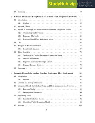
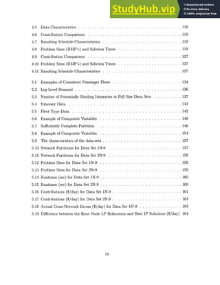
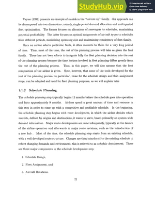
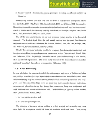
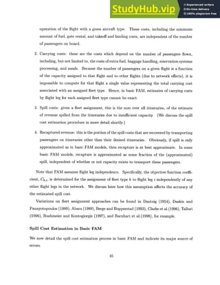
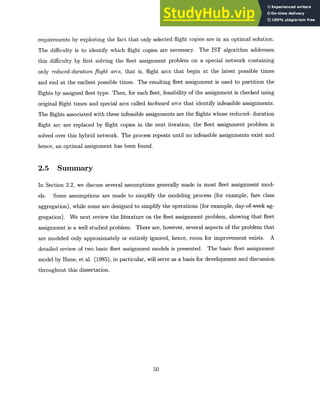
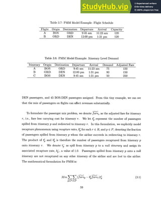
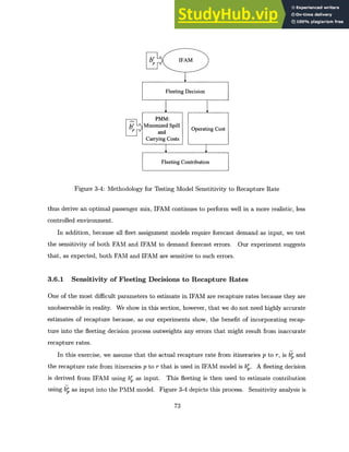
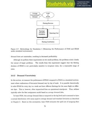
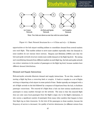
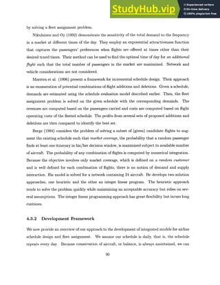
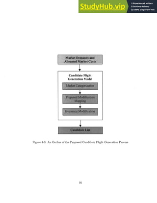
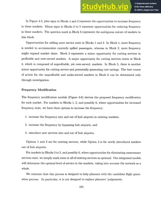
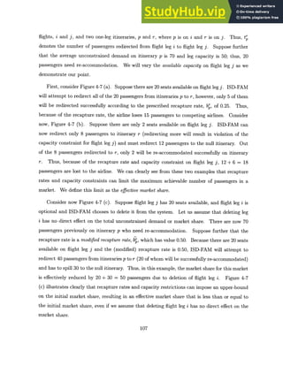
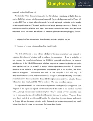
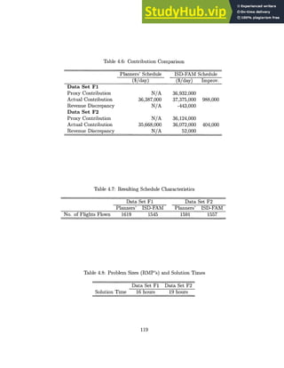
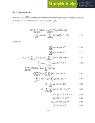
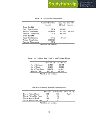
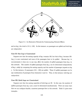
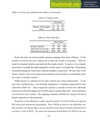
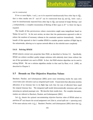
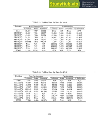
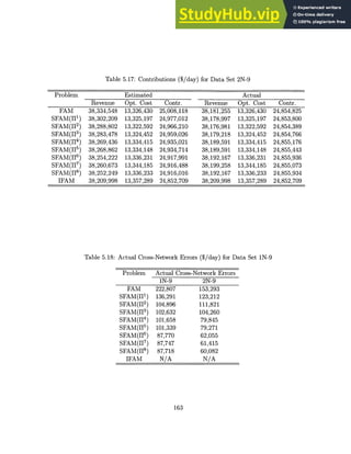
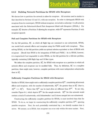
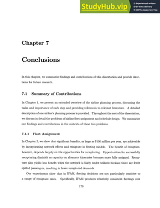
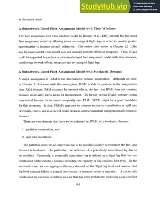
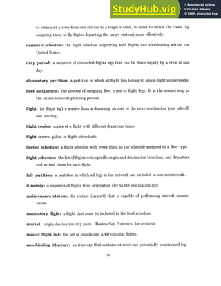
Note: br = 0.25 and b = 0.50
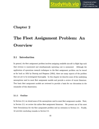
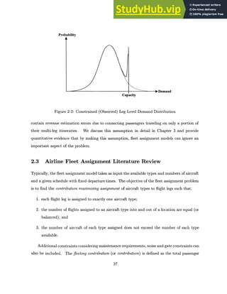
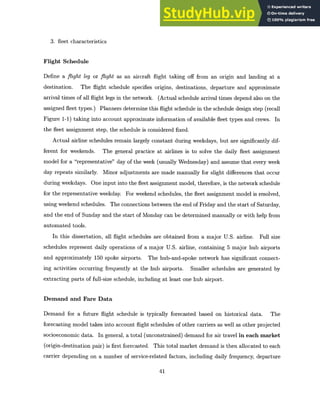
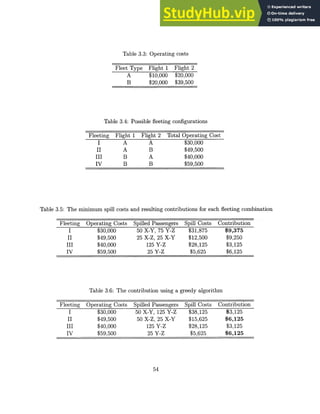
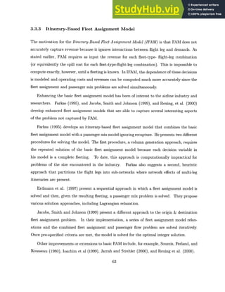
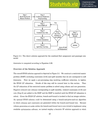
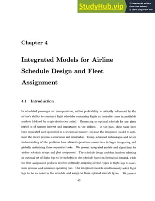
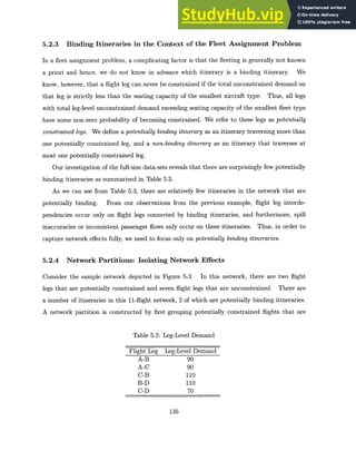
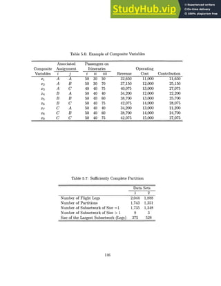
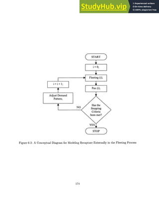
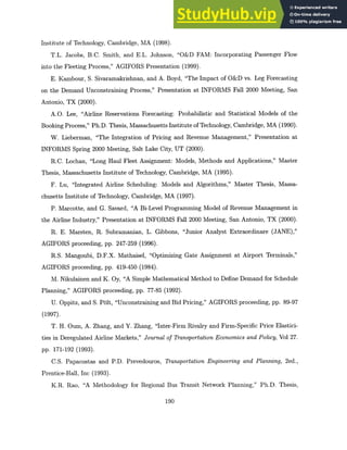
Figure 4-7: Indirect Effect of Recapture Rate and Capacity Constraint on Effective Market
Share
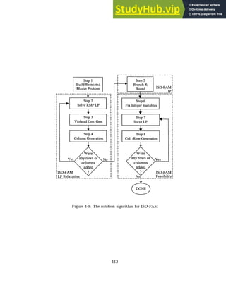
in that market. (For details, see Barnhart, Kniker, and Lohatepanont, 2001)
Mathematically, t' is the number of passengers being redirected from itinerary p to itinerary
r and bpt; is the number of passengers who are recaptured from itinerary p onto itinerary r. We
denote ti as spill from itinerary p to a null itinerary and assign its associated recapture rate,
b , a value of 1.0. Passengers spilled from itinerary p onto a null itinerary are not recaptured
on any other itinerary of the airline and are lost to the airline.
ISD-FAM utilizes recapture rates to capture (approximately) the interactions between de-
mand and supply. We demonstrate that although recapture rates do not alter total uncon-
strained demand (market share) in a market, capacity constraints on other itineraries and recap-
ture rates indirectly dictate the maximum number of passengers the airline can re-accommodate
within the system.
To see why, consider a market A-B in Figure 4-7. Suppose that there are two non-stop
106
b-t = 30
i: 70 extra
_passengers
A bt =20 B
j: 20 seats
available
Net Lost:
20 + 30 passengers

flights, i and j, and two one-leg itineraries, p and r, where p is on i and r is on j. Thus, t'
denotes the number of passengers redirected from flight leg i to flight leg j. Suppose further
that the average unconstrained demand on itinerary p is 70 and leg capacity is 50; thus, 20
passengers need re-accommodation. We will vary the available capacity on flight leg j as we
demonstrate our point.
First, consider Figure 4-7 (a). Suppose there are 20 seats available on flight leg j. ISD-FAM
will attempt to redirect all of the 20 passengers from itineraries p to r, however, only 5 of them
will be redirected successfully according to the prescribed recapture rate, b, of 0.25. Thus,
because of the recapture rate, the airline loses 15 passengers to competing airlines. Consider
now, Figure 4-7 (b). Suppose there are only 2 seats available on flight leg j. ISD-FAM can
now redirect only 8 passengers to itinerary r (redirecting more will result in violation of the
capacity constraint for flight leg j) and must redirect 12 passengers to the null itinerary. Out
of the 8 passengers redirected to r, only 2 will be re-accommodated successfully on itinerary
r. Thus, because of the recapture rate and capacity constraint on flight leg j, 12 + 6 = 18
passengers are lost to the airline. We can clearly see from these two examples that recapture
rates and capacity constraints can limit the maximum achievable number of passengers in a
market. We define this limit as the effective market share.
Consider now Figure 4-7 (c). Suppose flight leg j has 20 seats available, and flight leg i is
optional and ISD-FAM chooses to delete it from the system. Let us assume that deleting leg
i has no direct effect on the total unconstrained demand or market share. There are now 70
passengers previously on itinerary p who need re-accommodation. Suppose further that the
recapture rate is a modified recapturerate,b;, which has value 0.50. Because there are 20 seats
available on flight leg j and the (modified) recapture rate is 0.50, ISD-FAM will attempt to
redirect 40 passengers from itineraries p to r (20 of whom will be successfully re-accommodated)
and has to spill 30 to the null itinerary. Thus, in this example, the market share for this market
is effectively reduced by 20 + 30 = 50 passengers due to deletion of flight leg i. Figure 4-7
(c) illustrates clearly that recapture rates and capacity restrictions can impose an upper-bound
on the initial market share, resulting in an effective market share that is less than or equal to
the initial market share, even if we assume that deleting flight leg i has no direct effect on the
market share.
107

Thus, with recapture rates, ISD-FAM can indirectly capture the demand and supply inter-
actions by limiting the effective market share. More specifically, the resulting effective market
share depends on a number of factors:
1. recapture rates,
2. demand and fare on other itineraries, and
3. capacity assigned to other legs.
We show how we can capture demand and supply interactions more accurately in Section
4.7.
4.6.2 Objective Function
In this formulation, all average unconstrained itinerary demands are computed for the schedule
with all optional flights flown. The objective of ISD-FAM is to maximize schedule contribution,
defined as revenue generated less operatingcost incurred. The operating cost of a schedule, de-
noted 0, can be computed as EiCL >kEK Ck,ifk,i once fleet-flight assignments are determined.
The total revenue of a schedule can be computed from the following components:
1. initialunconstrainedrevenue (R),
R = farepDp, (4.1)
pCP
2. lost revenue due to spill (S),
S = fareptr,and (4.2)
pC~rCP
pep rep
3. recapturedrevenue from recapturingspilled passengers (M),
M =3[bgfarert. (4.3)
pEP reP
108

Equation 4.1 computes the initial unconstrained revenue for the schedule given uncon-
strained demand associated with all optional flight legs flown. Equations 4.2 and 4.3 measure
the changes in revenue due to spill and recapture, respectively. The contribution maximizing
objective function of ISD-FAM is therefore:
Max R-S+M-O. (4.4)
Given a fixed initial average unconstrained demand for the schedule, the initial uncon-
strained revenue (R) is a constant and we can therefore remove it from the objective function.
If we reverse the signs of the rest of the terms in Equation 4.4, we obtain an equivalent cost
minimizing objective function:
Min O + (S - M). (4.5)
Additional cost items that can be included are passenger related costs, which are composed
of , but not limited to,
1. passenger carrying costs (for example, meal, luggage handling), and
2. cost per revenue dollar (for example, reservation commission).
These cost items can be incorporated into the model by deducting them from the revenue
(or fare) obtained from a passenger. Thus, in the model, instead of using farep to denote
revenue obtained from a passenger traveling on itinerary p, we use fare, the net revenue from
a passenger traveling on itinerary p.
4.6.3 Formulation
We now present the formulation for the Integrated Schedule Design and Fleet Assignment
Model.
MinE S Ck,ifk,i + >3 (farep-bfare,)tr (4.6)
iGL kGK pEPrGP
109

Subject to:
E fk,i = 1 ,Vi E LF
kGK
Sfk,i < 1 ,Vi E LO
kEK
Yk,o,t- + fk,i - Yk,o,t+ - fk,i = 0 , V{k, o,t} E N
E Yk,o,tn + fk,i Nk ,Vk E K
OEA iECL(k)
S CAP fk,i + 6 't; -555 ft? Q
2 ,Vi E L
kcK rePpeP rCPpEP
r
rGP
< D , Vp E P
fk,i {0, 1} , Vk c
Yk,o,t 0 ,V{k, o, t}
t~ 0 ,Vp,r E P
K,Vi E L
E N
(4.7)
(4.8)
(4.9)
(4.10)
(4.11)
(4.12)
(4.13)
(4.14)
(4.15)
Constraints 4.7 are cover constraints for mandatory flights ensuring that every mandatory
flight is assigned to a fleet type. Constraints 4.8 are cover constraints for optional flights
allowing the model to choose whether or not to fly flight i in the resulting schedule; if flight
i is selected, a fleet type has to be assigned to it. Constraints 4.9 ensure the conservation of
aircraft flow. Constraints 4.10 are count constraints ensuring that only available aircraft are
used. Constraints 4.11 are capacity constraints ensuring that the number of passengers on each
flight i does not exceed its capacity. Constraints 4.12 are demand constraints ensuring that we
do not spill more passengers than demand for the itinerary.
4.6.4 Solution Approach
The accuracy of ISD-FAM hinges critically on the modified recapture rates, b 's, because they
are the only mechanism through which passengers can be reallocated. Thus, suppose we have
a correct set of modified recapture rates, solving ISD-FAM once will yield a solution to the
problem. This might not always be the case however, thus, we follow the approximate solution
110

approach outlined in Figure 4-8.
We initially obtain demand estimates for the full schedule (containing all flights from the
master flight list) using a schedule evaluation model. In step 1 of our approach in Figure 4-8,
we solve ISD-FAM to obtain a fleeted schedule. In step 2, a schedule evaluation model is called
to determine the new set of demands based on the schedule resulting from step 1. In step 3, we
evaluate the resulting schedule from Step 1 with revised demand from Step 2 using a schedule
evaluation model. In Step 4, we evaluate the schedule against the following stopping criteria:
1. magnitude of the improvement over planners' proposed schedule, and/or
2. closeness of revenue estimates from Step 1 and Step 3.
The first criteria can be used when a schedule for the next season has been prepared by
planners, the planners' schedule, and is available for comparison. If one is available, we
can compare the contributions between the ISD-FAM generated schedule and the planners'
schedule and if the ISD-FAM generated schedule generates a greater contribution, exceeding
some specified goal, we can stop with or without considering the second criterion. If a planners'
schedule is not available or the pre-specified improvement goal is not achieved, the second
criterion is triggered. The revenue from step 3 is then compared to that from step 1. If
they are close to each other, we have captured the changes in demand sufficiently well and the
procedure can be stopped; otherwise the modified recapture rates are revised using the demand
information from step 2, and ISD-FAM is resolved. The same procedure repeats.
No rigorous statements can be made about algorithmic convergence of this approach. Con-
vergence of the algorithm depends on the sensitivity of the model to the modified recapture
rates. Although we can control modified recapture rates, we cannot, however, control the num-
ber of passengers the model would redirect from one itinerary to another. Thus, we do not
have direct control of how the model handles the interactions between demand and supply.
In Section 4.7, we discuss an extended model that explicitly incorporates demand and supply
interactions, in which case we can control the interactions directly.
111

START
(1)
Solve ISD-FAM
4,
(2)
Calculate new demand for the
resulting schedule
(3)
Solve PMM with demand from
(2) and schedule from (1)
(4)
Has the
STOPPING
CRITERIA
been met
YES
STOP
(6)
Update
modified recapture rates
(5)
Identify itineraries that
cause discrepancies
A
NO
L
Figure 4-8: The Approximate Solution Approach
112
A
-1q
I

Step I Step 5
Build Restricted Branch &
Master Problem Bound D-FAM
IP
Step 2 Step 6
Solve RMP LP Fix Integer Variables
Step 3 Step 7
Violated Con. Gen. Solve LP
Step 4 Step 8
Column Generation Col. /Row Generation
Were Were
Yes any rows or No any rows or Yes
columns columns
added added
ISD-FAM ? ? ISD-FAM:
LP Relaxation _ No Feasibility:
DONE
Figure 4-9: The solution algorithm for ISD-FAM
113

Solution Algorithm for ISD-FAM
The algorithm for solving ISD-FAM is depicted in Figure 4-9. We first construct a restricted
master problem (RMP) excluding constraints 4.12 and spill variables (Inequalities 4.15) that
do not correspond to null itineraries. Then the LP relaxation of the restricted master problem
is solved using column and row generation. Negative reduced cost columns corresponding to
spill variables and violated constraints 4.12 are added to the RMP and the RMP is resolved
until the ISD-FAM LP relaxation is solved. Given the ISD-FAM LP relaxation, branch-and-
bound is invoked to find an integer solution. Once the ISD-FAM IP is solved, column and row
generation is again performed in order to obtain feasible passenger flows as integer variables are
fixed. (A small number of violated constraints might arise in the branch-and-bound tree.) An
optimal ISD-FAM solution could also be determined using a branch-and-price-and-cut algorithm
in which columns and constraints are generated within the branch-and-bound tree. Because
column generation at nodes within the branch-and-bound tree is non-trivial to implement using
available optimization software, we instead employ a heuristic IP solution approach in which
branch-and-bound allows column and row generation only at the root node and after the integer
solution is found.
4.6.5 Computational Experiences
We perform computational tests for ISD-FAM as outlined in Figure 4-10, assuming that it is
Period I and we are building a Period II schedule. Using a Period I schedule as our base
schedule, planners provide us with a master flight list including both mandatory and optional
flight legs. Using this master flight list, planners generate a proposed schedule for Period II,
the planners' schedule, which is used to evaluate ISD-FAM generated schedules. The planners'
schedule is, in fact, derived from actual Period II schedule (that was in operation) with some
minor modifications ensuring compatibility with our experiments.
We report ISD-FAM estimated contributions, called proxy contributions,based on demand
if all legs in the master flight list are flown. All three schedules are evaluated through a schedule
evaluation model, which accomplishes two tasks:
1. revises demands for Period II schedules, and
114

2. estimates actual contributionsusing estimated demands for Period II schedules, for that
schedule.
We call the contributions estimated by the schedule evaluation model actual contributions
to distinguish them from the proxy contributions. The difference between actual and proxy
contributions for a schedule measures the revenue discrepancy from inaccurately capturing
demand and supply interactions.
We perform our experiments on actual data including the planners' schedules, provided by a
major U.S. airline. Table 4.1 shows the characteristics of the networks in our two data sets. All
runs are performed on an HP C-3000 workstation computer with 2 GB RAM, running CPLEX
6.5.
Table 4.1: Data Characteristics
No. of Flight Legs No. of No. of No. of
Data Set Mand. Opt. Total Itineraries Fleets Aircraft
DI 645 108 753 60,347 4 166
D2 588 260 848 67,805 4 166
From Table 4.2, ISD-FAM generates significant improvements over the planner's schedule.
In data set D1 and D2, daily improvements of $582,521 and $729,120 are achieved respectively.
Assuming schedules repeat every day with similar demand for every day of the year, these
improvements translate into annual improvements of approximately $210 and $270 million. Like
in Chapter 3, these improvements do not necessarily represent actual improvements because
our experiments are performed in a controlled and limited environment. They should rather
be interpreted as upper bounds on the achievable improvements. Revenue discrepancies equal
$256,745 per day for data set D1 and $190,556 per day for data set D2, suggesting that if
demand and supply interactions could be more accurately modeled, even greater improvements
might be achieved.
Table 4.3 shows the problem sizes as well as the solution times for these two problems.
Table 4.4 presents the characteristics of the resulting schedules. It shows that ISD-FAM
achieves significant improvements through savings in operating costs (from operating fewer
flights) rather than through generating higher revenue. We also note that ISD-FAM schedules
115

Period I
Schedule
Planners' input
Master Flight List
Planners
I I
Period II I
Schedule
Schedule
Evaluation I
Model
Estimated
I I
I Contribution
Planners' Schedule
-- -- -- -- -- ---
ISD-FAM
I Period II
Schedule
II
II
Schedule
Evaluation I
Model
Estimated
I Contribution
I S
II
|IS__-ASchedule_
Figure 4-10: Testing Methodology
116

require significantly fewer aircraft to operate the schedule. Each aircraft removed from the
schedule represents significant savings to the airline because the airline can employ the aircraft
elsewhere, such as in new markets to increase profitability.
4.6.6 Full Size Problems
Table 4.5 gives the characteristics of 2 additional data sets tested. These data sets are accom-
panied by their associated planners' schedules. Notice that in both data sets, all flights are
optional. They represent full size problems at a major U.S. airline. The runs are performed
at a major U.S. airline using their implementation of our prototype ISD-FAM model, on a
6-processor computer, with 2 GB RAM, running Parallel CPLEX 6.
Table 4.6 summarizes the results of our model on full-size problems. In data set F1, the
ISD-FAM achieves a daily improvement of $988,000 over the planners' schedule. This translates
approximately to a $360 million per year improvement. In data set F2, the improvement is
smaller at $404,000 per day or $148 million per year. We note again that these are upper bounds
on the achievable improvements. In both of these data sets, ISD-FAM produces schedules that
operate fewer flight legs (Table 4.7).
We can clearly appreciate the complexity of these problems when we look at their solution
times, reported in Table 4.8. Note that these are runtimes on a 6-processor workstation,
running parallel CPLEX.
4.7 Schedule Design with Variable Market Share
In the previous section, we develop an integrated model for schedule design and fleet assignment
that approximately accounts for interactions between demand and supply. In this section,
we present the Extended Schedule Design and Fleet Assignment Model (ESD-FAM), in which
market shares are simultaneously updated as changes are made to the schedule. We present the
fundamental concept, model formulation, and solution algorithms. We compare and contrast
the model performance and solution quality of the approximate and more exact models.
117

Table 4.2: Contribution Comparision
Planners'
Schedule
($/day)
ISD-FAM
Schedule
($/day) Improv.
Data Set D1
Proxy Contribution N/A 1,999,094
Actual Contribution 1,159,828 1,742,349 582,521
Revenue Discrepancy N/A 256,745
Data Set D2
Table 4.3: Problem Sizes (RMP's) and Solution Times
Data Set Dl Data Set D2
No. of Columns 35,633 38,837
No. of Rows 2,999 3,326
No. of Non-Zeros 55,039 61,655
Solution Time 39 mins 78 mins
Table 4.4: Resulting Schedule Characteristics
Planners' Data Set DI Data Set D2
No. of Flights Flown 717 660 614
No. of Flights Not Flown 0 93 234
No. of Aircraft Used 166 154 148
No. of Aircraft Not Used 0 12 18
Table 4.5: Data Characteristics
No. of Flight Legs No. of No. of No. of
Data Set Mand. Opt. Total Itineraries Fleets Aircraft
F1 - 1993 1993 179,965 8 350
F2 - 1988 1988 180,114 8 350
118

Table 4.6: Contribution Comparison
Planners' Schedule ISD-FAM Schedule
($/day) ($/day) Improv.
Data Set F1
Revenue Discrepancy N/A -443,000
Data Set F2
Data Set F1 Data Set F2
Planners' ISD-FAM Planners' ISD-FAM
No. of Flights Flown 1619 1545 1591 1557
Solution Time
Data Set F1 Data Set F2
16 hours 19 hours
119

100 100 100
150 150+40 150+40+40
A 100 B A _100+20 B A B
100
(a) All itineraries (b) One optional (c) Two optional
operate itinerary is itineraries are
dropped dropped
1+ Mandatory Itineraries ----- * Optional Itineraries
x Unconstrained Itinerary Demand
Figure 4-11: Our Approach for Capturing Demand and Supply Interaction
4.7.1 An Explicit Treatment of Demand and Supply Interactions
Specific changes are made to the ISD-FAM model to allow for flight leg selection, and for
demand and supply interactions. Consider the example in Figure 4-11 (a), a market with 4
itineraries. The first and second itineraries are mandatory itineraries,that is, they contain
only mandatory flights. The third and fourth itineraries are optionalitineraries,that is, each of
these itineraries contains at least one optional flight. Let the first itinerary be in the morning
and the last three itineraries be in the afternoon.
The numbers on the arcs are the unconstrained demands (number of requests), Dp, when all
itineraries exist in the schedule. Thus, we assume that optional itineraries are initially flown.
Each itinerary has 100 requests except the second itinerary, which has 150 requests. (We can
view the second itinerary as a nonstop itinerary and the rest as connecting itineraries.) Hence,
there are a total of 450 requests when both optional itineraries are flown.
In Figure 4-11 (b), we assume that one of the optional flights in the last itinerary is deleted
and, as a result, the last itinerary no longer exists. At first glance, it may appear that 100
potential customers are lost. Some of these 100 potential customers, however, will go to other
airlines, and some will remain with the airline. Those that remain with the airline will request
other itineraries still in the schedule (itineraries 1-3 in this case). We assume that 40 and 20 of
120

the 100 requests previously on the fourth itinerary will request the second and third itineraries,
respectively. The first itinerary does not receive any additional requests because it is in the
morning and the 100 passengers prefer itineraries that depart close to the time (the afternoon)
of their original itinerary. The second itinerary receives more requests than the third because
the former is nonstop while the latter is connecting. Thus, the total requests for our airline are
now reduced to 410 with 40 requests lost to competitors.
In Figure 4-11 (c), we assume that the third itinerary is also deleted. The same phenomenon
occurs. The second itinerary receives 40 more requests from the 100 requests cancelled from
the third itinerary. The first itinerary again receives none. Now, the total request is reduced
to 330 with 120 requests lost in total. The lost requests when two itineraries are deleted more
than double those when only one itinerary is deleted.
This shows that our approach can capture the non-linear relationship between market share
and service frequency. We refer to the adjustments in demand resulting from changes in the
flight schedule as demand correctionterms. They correct the unconstrained demands for other
itineraries when optional itineraries are dropped. Specifically, the demand correction term,
AD~q, corrects demand on itinerary p when itinerary q is altered.
In our ESD-FAM formulation, demand correction terms for itinerary q, AD ,Vp E P are
applied depending on the itinerarystatus variable,Zq. Zq serves as a flag indicating whether or
not itinerary q is operated. Specifically, Zq equals 1 if itinerary q is operated and 0 otherwise.
Notice that itinerary q is operated only when all flight legs contained in q are operated. If one
or more flight legs in q are deleted, q is not operated. We show later in the formulation how
the value of Zq is specified.
Note that the corrections become approximate when there is more than one optional itinerary
deleted. To see why, consider again Figure 4-11 assuming as before that when an open itinerary
is cancelled, 40 requests will go to the nonstop itinerary, and 20 requests will go to the connect-
ing itinerary, for both itineraries 3 and 4. In Figure 4-11 (c), our approach predicts that the
total request is 330, based on the sum of the correction terms for cancellation of each itinerary,
one itinerary at a time. The total request of 330 approximates the true demand because the
combined effect of canceling two itineraries might exceed, or be less than, the sum of the in-
dividual effects of canceling one itinerary at a time. For example, if frequency in a market is
121

reduced below some critical threshold, market demand might decrease dramatically, far more
than the sum of the decreases brought about by considering deletion of only one itinerary p in
the schedule, for p drawn from a set of itineraries in a market. We explain how this problem
can be addressed, after presenting the model formulation.
4.7.2 Objective Function
Like in ISD-FAM, all average unconstrained itinerary demands are computed for the schedule
with all optional flights flown. Note that in ESD-FAM, we use ordinary recapture rates similar
to IFAM instead of the modified ones. The objective of ESD-FAM is to maximize schedule
contribution,defined as revenue generated less operatingcost incurred. The operating cost of
a schedule (0), initial unconstrained revenue (R), lost revenue due to spill (S), and recaptured
revenue from recapturing spilled passengers (M) can be computed as shown in Section 4.6. An
additional term is required, however, due to the introduction of demand correction terms:
changes in unconstrainedrevenue due to market share changes because of flight leg addition
or deletion (AR),
AR = (fareqDq- farepADP) - (1 - Zq). (4.16)
qEP
0
pEP:p:q
The term fareqDq is the total unconstrained revenue of itinerary q. The term EpEP:p~q
farepADS is the total change in unconstrained revenue on all other itineraries p () q) in the
same market due to deletion of itinerary q. Recall that Zq equals 1 if q is flown and 0 otherwise.
Thus, Equation 4.16 is the change in unconstrained revenue due to the deletion of itinerary q.
The contribution maximizing objective function of ESD-FAM is therefore:
Max R-AR-S+M-O. (4.17)
As in ISD-FAM, an equivalent cost minimizing objective function can be obtained by ignor-
ing the constant initial unconstrained revenue (R) and reversing the signs of all other elements
Min O+(S-M) +AR. (4.18)
122

4.7.3 Formulation
As in ISD-FAM, farep is used to denote the net revenue from a passenger travelling on itinerary
p. ESD-FAM can be formulated as shown in (4.19) - (4.31).
MinE E Ck,i fk,i + E ( ( -bpr--
Mm~~~~ >j> farep-bifarer)tpr
icL kcK pEP rEP
+ S (fareqDq - fareAD;)-(1 - Zq)
qCP
0
pGP:p~q
Sf= 1 ,Vi E LF
kcK
5 fi < 1 ,Vi E LO
kcK
Yk,o,t- +
iEI(k,o,t)
fk,i - Yk,o,t+ - fiA
iEO(k,o,t)
Yk,o,tn + >3 k,i
oEA iECL(k)
3 >3 6~iADP(1 - Zq) + E CAPkfk,i
pGPqEPO kEK
+ 6Pi
ot - bpbpb tp
rEPpEP rEPpGP
E AD{1 - Zq) + E tpr
qGPO rEP
Zq - 1 fk,i
kEK
Zq - Y , fk,i
iGL(q) kGK
= 0 ,V{k,o,t} E N
Nk ,Vk E K
Qi ,Vi E L
D, ,Vp E P
< 0 Vi E L(q)
> 1 - Nq ,Vq E P0
fk,i E {0, 1} ,Vk E K,Vi E L
Zq E {0, 1} ,Vq E P0
Yk,o,t 0 , V{k, o, t} E N
t; > 0 ,Vpr E P
123
Subject to:
(4.19)
(4.20)
(4.21)
(4.22)
(4.23)
(4.24)
(4.25)
(4.26)
(4.27)
(4.28)
(4.29)
(4.30)
(4.31)

Constraints 4.20 to 4.23 are similar to those of ISD-FAM. The term EqCPO AD(1 - Zq)
in Constraints 4.25 corrects the unconstrained demand for itinerary p E P when optional
itineraries q E P0 are deleted. Similarly, the term EpCP ZqePO 6p ADep(1 - Zq) in constraints
4.24 represents corrected demand but at the flight level. Constraints 4.26 - 4.27 are itinerary
status constraintsthat control the {0,1} variable, Zq, for itinerary q. Specifically, Constraints
4.26 ensure that Zq takes on value 0 if at least one leg in q is not flown and Constraints 4.27
ensure that Zq takes on value 1 if all legs in q are flown.
We stated earlier that demand corrections can be inaccurate when two or more itineraries
are cancelled at the same time. These inaccuracies can be obviated by adding another set of
{0,1} variables indicating the status of combinations of itineraries and associating additional
demand correction terms with these variables. For example, in Figure 4-11(c), we could add
a second order correction term to capture correctly the change in demands when the third
and fourth itineraries are both cancelled. Specifically, the number of requests for the second
itinerary would become 150+40+40+x, where x is the second order correction term associated
with cancellation of both the third and fourth itineraries. Note that x could take on either a
positive or negative value. Even though the addition of these variables is possible in theory,
the model can quickly become intractable in practice.
Passenger Flow Adjustment
Notice that ESD-FAM employs two mechanisms to adjust passenger flows:
1. demand correction terms, and
2. recapture rates.
Both accomplish the objective of re-accommodating passengers on alternate itineraries when
desired itineraries are not available, but with different underlying assumptions. To contrast,
consider itineraries p E P,q C P, and r E P in a market m. With demand correction terms,
ESD-FAM attempts to capture demand and supply interactions by adjusting the unconstrained
demand on alternate itineraries p E P in market m when an optional itinerary q E P0 (p 7 q) is
deleted, utilizing demand correction terms ADP's. In so doing, the total unconstrained demand
124

(market share) of the airline in market m is altered by Dq - peP:pQ.q ADq'. With recapture
rates, ESD-FAM attempts to reallocate passengers on alternate itineraries r E P in market m
when an itinerary p E P is capacitated, utilizing the recapture rates b's. This, however, does
not affect the total unconstrained demand (market share) of the airline in market m.
4.7.4 Solution Approach
The ESD-FAM model takes as input the master flight list, recapture rates, demand data,
demand correction terms, and fleet composition and size. In theory, an exact solution approach
can be outlined as shown in Figure 4-12. The idea is first to obtain exact demand correction
terms for as many combinations of flight deletions as possible, assuming all legs are initially
included. Higher order correction terms can be included if necessary. These correction terms
can be estimated using a schedule evaluation model. Then, ESD-FAM is solved, as outlined in
Section 4.6.4, to determine the optimal subset of flights to be flown based on the extensive set of
correction terms that are initially prepared. In theory, if we estimated exactly all higher-order
correction terms using a schedule evaluation model and included all of them in ESD-FAM, we
could find an optimal schedule by solving ESD-FAM once. This strategy is impractical, however,
because many runs of the schedule evaluation model (one run for each possible combination of
flight additions and deletions) are necessary to estimate the correction terms exactly.
Consequently, we adopt an approximate solution algorithm similar to that of ISD-FAM
outlined in Figure 4-8. Instead of trying to obtain exact demand correction terms at the
outset, we use rough estimates of these terms, revise them iteratively as we solve the problem
and add higher order correction terms as needed. Specifically, we solve ESD-FAM in Step 1,
and update the demand correction terms in Step 6. The algorithm for solving ESD-FAM itself
is similar to that for ISD-FAM, described in Section 4.6.4.
Convergence of the algorithm depends largely on the sensitivity of the model to demand
correction terms. If the model is very sensitive to these terms, it might take many iterations
to get them right, and higher-order correction terms might be necessary.
125

SSTART
Select subset of flights
Calculate demand correction
terms for selected subset of
flights using schedule
evaluation model
Have all possible
combinations of NO
flight additions
and deletions
been considered?
YES
Solve ESD-FAM
STOP
Figure 4-12: The Exact Solution Approach
126

Table 4.9: Contribution Comparison
Planners' Schedule ESD-FAM Schedule
($/day) ($/day) Improv.
Data Set D1
Data Set D2
Proxy Contribution N/A N/A*
Actual Contribution 1,159,828
Revenue Discrepancy N/A
*Solution not obtained
Data Set Dl Data Set D2
No. of Columns 48,742 65,447
No. of Rows 30,206 60,910
No. of Non-Zeros 164,676 34,4517
Solution Time 12.7 hrs 3+ days*
Planners' Data Set DI Data Set D2
No. of Flights Flown 717 668 N/A*
No. of Flights Not Flown 0 85
No. of Aircraft Used 166 157
No. of Aircraft Not Used 0 9
127

4.7.5 Computational Experiences
We perform an experiment similar to that for ISD-FAM, outlined in Figure 4-10. Tables 4.9
shows the results for data sets D1 and D2, respectively. The daily improvements shown
are measured against the planners' schedule for Period II. ESD-FAM generates considerably
improved schedules, with an increase in the actual daily contribution of $561,776. Assuming
that unconstrained demand is an average of daily demands and that the airline operates this
schedule 365 days, this daily improvement could translate to an improvement as large as $200
million per year. The discrepancy of $187,263 per day is observed. (Recall that in data set D1,
the discrepancy for ISD-FAM is $256,745.) This shows that ESD-FAM better captures demand
and supply interactions, resulting in smaller discrepancies. We cannot, however, achieve an
integer solution for data set D2 using ESD-FAM. Table 4.10 shows the size of the constraint
matrices and solution times for these problems. ESD-FAM on data set D2 ran for 3+ days
without achieving an integer solution, highlighting the increased difficulty of solving this model.
Table 4.11 presents the characteristics of the resulting schedule. ESD-FAM achieves signifi-
cant improvements through savings in operating costs (from operating fewer flights) rather than
through generating higher revenues. Additionally, the ESD-FAM solutions require significantly
fewer aircraft to operate the schedule.
As seen from this experiment, although ESD-FAM captures interactions between demand
and supply more accurately than ISD-FAM, it suffers from tractability issues for larger problems.
The additional demand correction terms significantly deteriorate solution performance.
4.8 Summary
In this chapter, we present two integrated models for airline schedule design and fleet assign-
ment:
1. the integrated schedule design and fleet assignment model (ISD-FAM), and
2. the extended schedule design and fleet assignment model (ESD-FAM).
ESD-FAM utilizes demand correction terms to adjust carrier market shares as schedules are
altered. ISD-FAM, on other hand, ignores these complicated interactions and instead utilizes
128

recapture rates to adjust demand, assuming constant market shares.
We present our computational experiences. Our preliminary results indicate that both ISD-
FAM and ESD-FAM are capable of producing improved schedules. ESD-FAM, however, could
suffer from tractability issues, particularly in larger size problems. In fact, as our experiments
show, ESD-FAM have difficulty solving medium size problems. In addition, data quality could
become an issue in ESD-FAM because its mechanism for adjusting demands requires very
detailed information on how market shares are affected when flight schedule changes. If good
quality data is not available, the more sophisticated method of capturing demand and supply
interactions might not be as advantageous. Thus, with current technology, ISD-FAM appears
to be the model of choice, primarily because of its improved tractability.
As shown in Section 4.6.6, ISD-FAM is capable of handling full-size U.S. domestic problems,
containing approximately 2,000 flight legs. The upper bounds on the improvements (compared
to a set of planners' solutions) are estimated to be as large as $100 million per year.
The scale and complexity of these problems cannot be ignored. These full size problems
can take as long as 20 hours to solve on a 6-processor workstation. In the next chapter, we
revisit the fleet assignment model and develop an alternative formulation that models network
effects and recapture in a manner allowing it to be solved more easily, and possibly expanded
and applied to schedule design.
129

Chapter 5
Alternative Formulation for the
Airline Fleet Assignment Problem
5.1 Introduction
In Chapter 3, we discuss at length the importance of network effects and recapture in the
fleet assignment problem and quantify the potential benefit of modeling them in the itinerary-
based fleet assignment model (IFAM). In Chapter 4, we present integrated models for schedule
design and fleet assignment. There are strong interests in industry and academia to further
integrate the planning process (outlined in Figure 1-1) in order to achieve global optimality.
Although our models do well on these problems, they appear to be hitting the limits in terms
of solvability and tractability as seen, in particular, in the schedule design problem. Thus,
unless there are significant breakthroughs in computational technologies and/or optimization
techniques, we anticipate difficulties in further extending IFAM to include other aspects of the
planning process.
In this chapter, we investigate the nature of network effects and derive a new approach to the
airline fleet assignment problem. In particular, we build an alternative fleet assignment model,
in which network effects can be conveniently modeled without sacrificing as much solvability
and tractability as in IFAM. The intention is to provide a new model that can serve as a
kernel for further integration of other planning steps. Throughout this chapter, we limit our
discussion only to simplified cases without recapture, unless noted otherwise. In Chapter 6,
131

we present a detailed approach incorporating recapture as well as other extensions.
5.1.1 Outline
In Section 5.2, we investigate network effects on the fleet assignment problem and present
significant observations, which are formalized in Section 5.3. We introduce the idea of our
proposed model in Section 5.4 and present the model in Section 5.5 In Section 5.6, we detail
implementation related issues, including column enumeration. We describe an important
property of the model in Section 5.7. Finally, our computational experiences are presented in
Section 5.8.
5.2 Network Effects: A Closer Look
Recall from Chapter 3 that due to flight leg interdependencies, or network effects, spill inac-
curacies arise when spill is estimated for a flight leg independently of other flight legs in the
network. Specifically, such inaccuracies occur because conservation of passenger flow require-
ments are ignored. The itinerary-based fleet assignment model explicitly enforces consistent
passengerflow, passenger flow that honors conservation of flow, through its use of traffic vari-
ables (recall Chapter 3), thus achieving more accurate spill estimation. In this section, we
investigate more closely the flight leg interdependencies and demonstrate through an example,
when such interdependencies matter and when they do not.
5.2.1 Example: Consistent Passenger Flow and Flight Leg Interdependency
(Network Effects)
Consider the sample network depicted in Figure 5-1. There are 2 flight legs, i and j, serving
three cities, A, B, and C. Passengers can travel on three itineraries: i (A-B), ii (A-C, connecting
through B), or iii (B-C). Suppose that the numbers of travellers requesting itineraries i, ii,
and iii are 50, 40, and 75 respectively. Consider the following three cases.
Case I: Both Legs are Unconstrained
Suppose that the seating capacities of legs i and j are 100 and 150 respectively. It is clear
that both legs are unconstrained because on leg i the total number of requests is 90 (< 100)
132

40
(N (Wi)
50 75
A B C
Figure 5-1: An Illustrative Network for Understanding Network Effects
and on leg j the total is 115 (< 150). In this instance, no passengers are spilled and both legs
are independent.
Case II: One Leg is Constrained
Suppose now that the seating capacity of leg i remains 100, but that of leg j becomes 100.
Leg j is now constrained and some of the passengers have to be spilled. Because leg i is
unconstrained, it does not, in any way, affect the number of spilled passengers from leg j in
this network. The number of spilled passengers from leg j can be determined independently
of leg i, solely by comparing the seating capacity and the number of passenger requests on leg
j. In this instance, 15 passengers (115 - 100) are spilled. These 15 spilled passengers can be
any combination of passengers from itineraries ii and iii. Thus, in this instance, both legs are
independent.
Case III: Both Legs are Constrained
Suppose now that the seating capacities of both legs are 80. In this case, the numbers of
spilled passengers from leg i and j must be determined simultaneously. There are many ways
that we can configure feasible, consistent passenger flow in this network. Table 5.1 gives some
examples.
133

It is clear from Table 5.1 that consistent flows of passengers can be achieved, in this instance,
only by considering capacities and demands on both legs i and j simultaneously, therefore legs
i and j are interdependent,that is, there are network effects in this network.
Notice that the only parameters that change in our example are capacities of legs i and
j. In particular, because of changes in capacities, the status of flight legs change from uncon-
strained to constrained. Flight leg interdependencies arise only when both legs in our example
become constrained. In other words, network effect matter only when there are passengers
traveling on itineraries that traverse multiple constrained legs. We denote such itineraries as
binding itineraries. Similarly, non-binding itinerariesare itineraries that traverse at most one
constrained leg, for example, itinerary ii in Case II of the example earlier.
5.2.2 Network Mapping
In this section, we introduce a special network mapping that will greatly facilitate our discussion
for the remainder of the chapter. Consider the network depicted in Figure 5-2 (i) consisting of
4 cities served by 5 flight legs. Suppose that the capacity on each flight leg is 100. There are
8 distinct itineraries in this network-5 non-stop, 2 one-stop, and 1 two-stop. Their demands
are shown in the figure. The demand on each leg is reported in Table 5.2.
Based on the prescribed demands, there are two constrained legs, namely, C-B and B-D,
depicted in Figure 5-2 (ii). Figure 5-2 (iii) and (iv) introduce the transformation from the node-
arc network into our graphical representation. Specifically, flight legs, which previously were
denoted as links, are transformed into nodes; and (connecting) itineraries now become links
connecting nodes. In Figure 5-2 (iv), binding itinerary (A-C-B-D) and non-binding itineraries
(A-B-D and A-C-D) are differentiated.
Table 5.1: Examples of Consistent Passenger Flows
Passengers on Passengers on
Scenario Itin. i Itin. ii Itin. iii Leg i Leg j
(a) 50 30 50 80 80
(b) 40 40 40 80 80
(c) 50 5 75 55 80
134

(i)
B
A D
C
Capacity on Each Leg is 100
B
C
Constrained Leg
Unconstrained Leg
(ii)
B
Constrained Leg
Unconstrained Leg
--- CB indg Itinerary
- - - Non-Binding Itinerary
Figure 5-2: An Example of Network Mapping
135
Itineraries Demand
50
90
40
20
20

5.2.3 Binding Itineraries in the Context of the Fleet Assignment Problem
In a fleet assignment problem, a complicating factor is that the fleeting is generally not known
a priori and hence, we do not know in advance which itinerary is a binding itinerary. We
know, however, that a flight leg can never be constrained if the total unconstrained demand on
that leg is strictly less than the seating capacity of the smallest aircraft type. Thus, all legs
with total leg-level unconstrained demand exceeding seating capacity of the smallest fleet type
have some non-zero probability of becoming constrained. We refer to these legs as potentially
constrainedlegs. We define a potentially binding itineraryas an itinerary traversing more than
one potentially constrained leg, and a non-binding itinerary as an itinerary that traverses at
most one potentially constrained leg.
Our investigation of the full-size data sets reveals that there are surprisingly few potentially
binding itineraries as summarized in Table 5.3.
As we can see from Table 5.3, there are relatively few itineraries in the network that are
potentially binding. From our observations from the previous example, flight leg interde-
pendencies occur only on flight legs connected by binding itineraries, and furthermore, spill
inaccuracies or inconsistent passenger flows only occur on these itineraries. Thus, in order to
capture network effects fully, we need to focus only on potentially binding itineraries.
5.2.4 Network Partitions: Isolating Network Effects
Consider the sample network depicted in Figure 5-3. In this network, there are two flight
legs that are potentially constrained and seven flight legs that are unconstrained. There are
a number of itineraries in this 11-flight network, 2 of which are potentially binding itineraries.
A network partition is constructed by first grouping potentially constrained flights that are
Table 5.2: Leg-Level Demand
Flight Leg Leg-Level Demand
A-B 90
A-C 90
C-B 110
B-D 110
C-D 70
136

connected by potentially binding itineraries, resulting in Subnetworks 1 and 2. Each of the
remaining flight leg corresponds to a single-flight subnetwork, as in Subnetworks 3 to 9.
Network effects can potentially occur only on flight legs that are connected through po-
tentially binding itineraries. In our sample network, 2 potentially binding itineraries connect
4 potentially constrained legs, but only 2 of these legs are connected to another leg through
potentially binding itineraries (see Figure 5-3). These subnetworks are independent. That is,
consistent passenger flows for the entire network can be determined by constructing consistent
passenger flows for each subnetwork.
To see why, consider Subnetwork 1 in Figure 5-3, two potentially constrained legs are con-
nected through a potentially binding itineraries. Passenger flow on this potentially binding
itinerary must be determined by considering simultaneously both legs included in Subnetwork
1 to ensure consistency. There are 4 other flight legs connected to this subnetwork through 4
non-binding itineraries. All of these legs are unconstrained, thus consistent passenger flows on
the 4 non-binding itineraries connecting Subnetwork 1 can be determined solely from flight legs
in Subnetwork 1. (Recall Case II of the passenger flow example.) Consider now Subnetwork
4, which contains one unconstrained leg. Because it is unconstrained, no inconsistent flow can
occur from this leg.
Thus, network effects are fully contained within each subnetwork shown in Figure 5-3, with
each subnetwork isolated from all others. In other words, each of the 9 subnetworks in Figure 5-
3 is spill-contained. Hence, spill can be determined accurately by considering each subnetwork
independently. The total spill of the entire network is the summation of spills from these
independent subnetworks.
Table 5.3: Number of Potentially Binding Itineraries in Full Size Data Sets
Data Set
1 2
Number of Legs 2044 1888
% of potentially constrained legs 17% 30%
Number of Itineraries 76,741 75,484
% of potentially binding itineraries 2% 6%
137

>12.
------
A"
Potentially
Constrained
Flight Leg
- -
Unconstrained
Flight Leg
Potentially
Binding
Itinerary
"""'"Non-Binding
Itinerary
Figure 5-3: Network Partition
138

5.2.5 Summary
In FAM, each flight is itself a subnetwork and thus, network effects cannot be captured. In
IFAM, we can think of the entire network as a subnetwork and all network effects are contained
in this subnetwork. In Figure 5-3, we illustrate that network effects can be contained in
several intelligently constructed subnetworks. In the next section, we describe in detail how
we partition the network to isolate network effects.
5.3 Network Partitioning
The key to isolating network effects successfully is network partitioning. Although there are
numerous ways to partition a network, we are interested in partitions that can efficiently and
sufficiently isolate network effects. In this section, we formalize the idea of network partitioning
and present our partitioning approach.
5.3.1 Mathematical Representation
To facilitate our descriptions, we introduce some additional notation. HS denotes a network
partition for a given network N; L is the set of flight legs in the flight schedule indexed by i,
LI = I; and Srs is the set of subnetworks in a partition Hs indexed by m, ISns I= Ms.
A partition HS decomposes L (= {L 2 ,i = 1, ...,I}) into mutually exclusive and collectively
exhaustive subnetworks Sgs c Srs, m = 1, ..., MS, where n' = |S1sl. Mathematically,
exh austivU
sub ne work S;SrV '
Us= S.S: SgS C SCS, m =1,...,M s,s s n ss =$,Vm n. Fur-
M=1
ther, Sg = {(Li)1, (Lj) 2 ,..., (Lk)nm Ii # j k} and S1 s = L.
To illustrate, consider again the network in Figure 5-3. In this network I = 11, and L =
{L1 , L2 , ..., Lil} A partition Hs decomposes L into 9 subnetworks, or Hs = {S' S2 S 9
Further, IS'sl = ns =2, S =n s=2,and JS =js njs =1,m=3 ...
9.
Nesting of Network Partitions. A partition HS is nested in partition IT when every
member of Hs is a member of 1 T (H9 +- S C ST, VSIls E S1S, VST E Sfr).
Notice that if fIS -< g, then MS > MT, and equivalently, if fiS _< 1 1 T, then MS > MT.
139

Further, 1S < 1 T is termed as IS is finer than HT, or equivalently as IT is more consolidated
than HS.
5.3.2 Elementary, Full, and Complete Partitions
We define an elementary partition,H0
, as a partition in which each subnetwork S;o consists of
exactly one flight leg. Note also that M 0
= I. We define a full partition,HF, as a partition
in which each flight leg belongs to exactly one partition, S, Notice that H' < HF, for any
partition HS
A complete partition, 1c, is one in which all network effects are captured fully by the
independent subnetworks. One extreme example of a complete partition is the full partition.
Oftentimes there exists a sufficiently complete partition, HSC -< 1 C, in which all network
effects can be captured but MSC >> Mc. The partition in Figure 5-3 is an example of a
sufficiently complete partition. A sufficiently complete partition can be constructed by placing
in a common subnetwork all potentially constrained legs that are connected through potentially
constrained itineraries. All other legs that are not connected to other legs are, by construction,
not connected to other constrained legs through potentially binding itineraries and hence, can
be contained in single-leg subnetworks.
5.4 An Alternate Formulation for the Fleet Assignment Prob-
lem
In this section, we compare and contrast the fleet assignment models presented in previous
chapters beginning with the basic (leg-based) fleet assignment model to the itinerary-based
fleet assignment model, and introduce the idea of our proposed model.
Leg-Based Fleet Assignment
The basic fleet assignment model (FAM) reviewed in Chapter 2 is a leg-based fleet assignment
model, built on the flight leg independence assumption. This assumption that flight leg i in
the network is independent from all other legs j implies that the passenger flow on leg i can be
determined solely from comparing its requests and capacity. Associated with each fleet-flight
140

assignment variable, fki, is thus an estimate of the contribution of i, given that a fleet type k
is assigned to it and consistent passenger flows are ignored.
Itinerary-Based Fleet Assignment Model
The itinerary-based fleet assignment model (IFAM) reviewed in Chapter 3 addresses the incon-
sistent passenger flow issue of the basic fleet assignment model by explicitly modeling itinerary-
level passenger flows. In this way, the supply side of the problem is modeled through the
fleet-flight assignment variables and the demand side is modeled with the traffic variables.
These traffic variables ensure consistent passenger flows across the network.
Subnetwork-Based Fleet Assignment Model
Our proposed formulation, called the Subnetwork-Based Fleet Assignment Model (SFAM), can
be viewed as being intermediate between FAM and IFAM. The basic idea behind SFAM is
to take into account accurate passenger flow information without explicitly modeling traffic
variables.
In the fleet assignment problem, we do not know a priori what the fleetings are. In other
words, there are two types of decisions that the model has to make simultaneously: fleet type,
flight leg assignment and corresponding consistent passenger flows over the networks. One
approach, similar to that of IFAM, is to model both types of decision variables explicitly.
Introducing traffic variables into the fleet assignment model has adverse effects on the strength
of the fleet assignment formulation, resulting in a fractionality issue, as shown in Barnhart,
Kniker, and Lohatepanont (2001). Another approach is to use composite variables (Armacost,
2000) to model both types of decision variables simultaneously. Armacost (2000) observes that
composite variable models have strengthened LP relaxation behavior, facilitating the solution
of large problems.
The basic idea of the composite variable approach is to bundle different types of decision
variables together and represent them simultaneously as one type of decision variable in the
formulation. In our application, two types of decision variables, fleet-flight assignment and
passenger flow, can be bundled together as shown in the following example. Consider again
Figure 5-1, in which two flight legs, i and j, can accommodate three itineraries, i, ii, and iii.
141

Tables 5.4 and 5.5 give additional data related to this example.
Table 5.4: Itinerary Data
Itineraries
i ii iii
Number of Passengers 50 40 75
Fares 200 380 225
Table 5.5: Fleet Type Data
Fleet Types
A B C
Seating Capacity 80 100 120
Operating Cost for leg i 5000 6000 7000
Operating Cost for leg j 6000 7000 8000
Recall that there are several possible consistent passenger flows given a fleeting. In this
example, we will use the most common one in which the revenue is maximized. Table 5.6
shows the composite variables associated with this sample network. In essence, it is a complete
enumeration of possible fleet-flight assignments of 3 fleet types to two flight legs. Enumerating
all possible fleetings for subnetworks in full-size problems is impractical. We show later in this
chapter, however, that we can exploit certain properties of the problem to substantially reduce
the number of variables required.
SFAM operates on partitions of the entire network (into several subnetworks). In the
most basic implementation, a set of feasible assignments is completely enumerated for each
subnetwork (Table 5.6). These assignments represent a mutually exclusive and collectively
exhaustive set of feasible assignments of all fleet types to member flight legs. Such enumeration
is performed on every network. The assignment variables of SFAM thus comprise the sets of
feasible assignments of all subnetworks.
Recall that in the sufficiently complete network partition, all network effects are captured
fully within each subnetwork independently. Thus, if SFAM is solved on the sufficiently com-
plete partition, all network effects can be captured and the optimal solution achieved will be
equivalent to that of IFAM. We present the mathematical formulation for SFAM in the next
142

section.
5.5 The Subnetwork-Based Fleet Assignment Model Formula-
tion
In this section, we present the formulation for the subnetwork-based fleet assignment model.
Suppose that SFAM is solved on a partition HS, where 11S = Ms. For each subnetwork
Sgs C S11s, a set of assignments of fleet types to member flight legs can be enumerated. Each
assignment is denoted (fgjs)i. Let Frjs be the set of all feasible assignment of fleet types to
member flight legs and IFrSI =rq's. Thus, FgS =
The formulation of SFAM is structurally similar to that of FAM (Hane et al., 1995). The
only difference is how the assignment variables are handled. To facilitate our presentation, we
repeat the FAM formulation:
Min Ck,ifk,i (5.1)
iEL kEK
Subject to:
fZ,i = 1,Vi E L (5.2)
kcK
Yk,o,t- + fk,i - Yk,o,t+ - fk,i = 0, Vk, o, t (5.3)
iEI(k,o,t) icO(k,o,t)
Yk,o,tm + E fk,i <_ Nk,Vk E K (5.4)
ocA iECL(k)
fk,i E {0, 1},Vk E KVi E L (5.5)
Yk,o,t > 0, Vk, o, t (5.6)
Notice that in FAM, the assignment variable, fk,i, represents the assignment of fleet type k
to flight leg i. In SFAM, the assignment variable, (fgs)n, represents an assignment of fleet types
to member flight legs of subnetwork m (Sps) in partition S (HS). SFAM can be formulated
as follows:
143

MS m/J
Min (rs)"(fs) (5.7)
m=1 n=1
Subject to:
Ms 77rs
( ( = 1 ,Vi E L (5.8)
m=1 n=1
Ms
Yk,o,t- + E S MI
(K n IIr
iEI(k,o,t) m=1 n=1
-Yk,o,t+ - (n)k'i(frs) = 0 ,Vk,o,t E N (5.9)
iEO(k,o,t) m=1 n=1
MS 77?
Yk,o,tm + (5s ) (fs)_ Nk ,Vk E K (5.10)
oGA icCL(k) m=1 n=1
rs 0,1} ,Vn E F;5 ,Vm E S (5.11)
Yk,o,t 0 ,V{k, o, t} E N (5.12)
Similar to FAM, the objective function coefficient, (CMS), in SFAM represents assignment
cost (the sum of spill and operating costs). Unlike FAM, however, in SFAM these assignment
costs are accurate if SFAM is solved on a complete partition. Recall that in a complete
partition, network effects can be isolated into independent subnetworks and the total network
effect is the sum of assignment costs for each subnetwork.
The objective function shown (Equation 5.7) is to minimize the assignment cost. An equiv-
alent contribution-maximization objective function can be written using similar mathematical
manipulation shown in Section 4.6.2. Except the assignment variables, all other components
of SFAM match closely those in FAM. Equations 5.8 are the cover constraints ensuring that
every flight leg is covered by one fleet type. (6ms)' equals 1 if instance n of subnetwork m in
partition HS covers flight leg i, and 0 otherwise. Equations 5.9 are the conservation of aircraft
flow constraints. (K m )k ' equals 1 if instance n of subnetwork m in partition JS covers flight
leg i with fleet type k, and 0 otherwise. Equations 5.10 are the aircraft count constraints.
(Hs ) is the number of times instance n of subnetwork m in partition HS crosses the count
144

line with fleet type k.
5.5.1 Strength of SFAM Formulation
Barnhart, Farahat, and Lohatepanont (2001) show that SFAM and IFAM models are equivalent
and that the LP relaxation of SFAM is strictly stronger than that of IFAM. The implication
of the latter property to model solvability is demonstrated in Section 5.8.
5.6 Solution Approach
In this section we provide details of our SFAM implementation. There are two primary chal-
lenges:
1. partition construction, and
2. column enumeration.
The first concerns effective partition building because solving a complete partition on a full-
size problem is impractical. The second challenge arises from the fact that SFAM solvability
is linked to the constraint matrix size. Complete enumeration of all possible fleetings in all
subnetworks adversely affects the effectiveness and efficiency of SFAM greatly. We provide
an effective way to enumerate only necessary columns, exploiting certain characteristics of the
problem. We show that our approach for enumerating columns reduces the number of necessary
columns tremendously. Lastly, we give an overview of a solution approach to SFAM.
5.6.1 Partition Construction
The sufficiently complete partition can be constructed as outlined in Section 5.3. If SFAM
can be solved on the sufficiently complete partition, an optimal solution equivalent to that of
IFAM is achieved. Solving SFAM on the sufficiently complete partition, however, is typically
impractical, if not impossible.
Table 5.7 depicts subnetwork characteristics of the sufficiently complete partition on two
full-size problems. We can see from Table 5.7 that a significant portion of the network is not
affected by flight leg interdependencies (1,735 and 1,348 legs in Data Sets 1 and 2, respectively).
145

Table 5.6: Example of Composite Variables
Associated Passengers on
Composite Assignment Itineraries Operating
Variables i j i ii iii Revenue Cost Contribution
X1 A A 50 30 50 32,650 11,000 21,650
X2 A B 50 30 70 37,150 12,000 25,150
X3 A C 40 40 75 40,075 13,000 27,075
X4 B A 50 40 40 34,200 12,000 22,200
X5 B B 50 40 60 38,700 13,000 25,700
X6 B C 50 40 75 42,075 14,000 28,075
X7 C A 50 40 40 34,200 13,000 21,200
xs C B 50 40 60 38,700 14,000 24,700
X9 C C 50 40 75 42,075 15,000 27,075
Table 5.7: Sufficiently Complete Partition
Data Sets
1 2
Number of Flight Legs 2,044 1,888
Number of Partitions 1,743 1,351
Number of Subnetwork of Size =1 1,735 1,348
Number of Subnetwork of Size > 1 8 3
Size of the Largest Subnetwork (Legs) 275 528
146

Largest
Subnetwork
(275 Legs)
Data Set 1
Largest
Subnetwork
(528 Legs)
Data Set 2
Figure 5-4: Graphical Representation of the
Data Sets
Sufficiently Complete Partition in Two Full-Size
The difficult fact is that 275 out of the 309 remaining legs left in Data Set 1 are connected,
forming a huge subnetwork. Data Set 2 suffers from the same problem. Figure 5-4 illustrates
the situation graphically. The number of possible fleeting combinations is bounded by K",
where K is the number of fleet types and n is the number of members in the subnetwork.
Thus, practicality prevents us enumerating all possible fleeting combinations for subnetworks
of the sizes depicted in Figure 5-4. Our idea is to break-up large subnetworks in the sufficiently
complete partition into several manageably sized subnetworks, as shown in Figure 5-5.
Subdividing the Sufficiently Complete Partition
In our implementation, available computer memory dictates how many columns we can
include in our model. Because problem size grows exponentially with the number of legs
included in the subnetwork, we can limit problem size by restricting the maximum number of
flight legs allowed in each subnetwork.
147

Breaking Large
Subnetwork into
Several Managable Size
Subnetworks
Figure 5-5: Graphical Representation of Our Approach
To facilitate the understanding of our approach, consider Figure 5-6 as an example. Sub-
network 6 in the upper picture contains 6 constrained legs. Suppose that there are 10 fleet
types in this problem. A complete enumeration of the possible fleetings in this subnetwork
results in 1 million variables, which is impractical. Thus, we limit the maximum size of our
subnetwork to 4 flight legs (or equivalently 10,000 variables) in this example. Our objective
then is to subdivide Subnetwork 6 in the upper picture of Figure 5-6 into smaller subnetworks,
each of which is smaller than 4 flight legs.
To do this, recall that constrained legs in any subnetwork are connected together by poten-
tially binding itineraries. If we break some of these potentially binding itineraries some of the
previously connected constrained legs will become disconnected. This is shown in the lower
picture of Figure 5-6, in which one of the potentially binding itineraries is broken, resulting in
disconnecting the two constrained legs. Note that in actuality, a pair of constrained legs in a
subnetwork are often connected by more than one potentially binding itinerary. Thus, in order
to break the link, all of the potentially binding itineraries connecting the two flight legs have
to be broken.
By separating a pair of previously connected, potentially constrained legs, we in effect allow
148

3--'
5-
UnconstrainedI-- -- NnBidn
%2
/
Potentially Potentially
Constrained - Binding
Flight Leg Itinerary
Unconstrained b Non-Binding
Flight Leg Itinerary
Broken
........ Potentially
Binding
Itinerary
Figure 5-6: Subdividing a Subnetwork by Breaking the Potentially Binding Connection
149

some inconsistent passenger flow to occur. To see why, suppose that both legs actually become
constrained. The passengers traveling on the binding and previously connected but now broken
itineraries are handled independently in the two subnetworks. SFAM can account fully only
for network effects occurring within subnetworks, not across subnetworks. Thus, SFAM will
not be able to capture network effects should they occur amongst these two flight legs.
Breaking Potentially Binding Itineraries
As shown earlier, there is a trade-off in subdividing the sufficiently complete partition. The
finer we subdivide the sufficiently complete partition, the easier the problem is to solve but we
capture fewer network effects. We can, however, manage this trade-off. Specifically, we can
manage the error from disconnecting potentially binding itineraries by carefully selecting the
potentially binding itineraries to be disconnected.
Consider Figure 5-7, a pair of potentially constrained legs, i and j, is connected only by a
potentially binding itinerary p, which traverses a total of 4 legs. In order to disconnect i and
j, we have to break p into 2 fictitious independent itineraries-one traveling on i (and another
up-line leg) and the other on j (and another down-line leg). We maintain the total number of
passengers and revenue associated with these passengers in the split itineraries. For example,
in Figure 5-7, both q and r have requests of 20 passengers each. The fares associated with q
and r are a combination of individual fares that sum to the original $200 fare. In this example,
the worst case scenario in terms of revenue miscalculation, is the following:
* 20 seats are allocated on flight leg j for passengers on fictitious itinerary r, and
* no seats are allocated on flight leg i for passengers on fictitious itinerary q.
This can happen because the fictitious itinerary r has associated with it a rather high fare
of $125, while the other fictitious itinerary, q, has rather low fare associated with it. If this
happens, none of the passengers on itinerary p will be carried, because seats are not reserved
for them on flight leg i. Thus, the revenue miscalculation is $125 . 20 = $2,500. The largest
miscalculation, however, happens when all of the fare is associated with leg j (or i) and none
150

BEFORE
20 Passengers
$200 Fare
P
AFTER r 20 passengers
$125 fare
r
. 20 passengers
$75 fare
Figure 5-7: Breaking A Potentially Binding Itinerary
to the other, in which case, the miscalculation can be as high as $4, 000, the total revenue
associated with itinerary p.
Thus, the itinerary-level cross-network error,the most error that we incur from breaking a
potentially binding itinerary, is the total revenue associated with that itinerary, i.e., the product
of unconstrained demand and its fare. Recall that there can be many potentially binding
itineraries connecting two potentially constrained legs; thus, the total error from disconnecting
two potentially constrained legs in a subnetwork is the sum of all itinerary-level cross-network
errors, or link-level cross-networkerror. We formally define a link as the collection of potentially
binding itineraries connecting two potentially constrained legs. There could be many links
that have to be broken, in order to subdivide a subnetwork; thus, the subnetwork-level cross-
network error,the summation of link-level cross-network error of all links broken, represents
the maximum error that we can incur from subdividing a subnetwork. Figure 5-8 depicts these
151

ItineraryLevel
Link Level
Subnetwork Level
%
I
/*
/*
%/
Figure 5-8: Three Levels of Possible Subnetwork Division
three levels.
Algorithms for Subdividing Subnetworks
For any given subnetwork, in order to minimize the impact on miscalculation of network
effects, we should subdivide along the set of links that yield minimum subnetwork-level cross-
network error. This can be conveniently formulated as a minimum cut optimization subprob-
lem, where the cost of a link is the link-level cross-network error. We can subdivide a large
subnetwork in two ways:
1. given a pre-specified maximum subnetwork size, subdivide a given subnetwork once into
152

several subnetworks of sizes smaller or equal to the pre-specified maximum size, or
2. iteratively subdivide a given subnetwork along the minimum cut (each iteration subdi-
vides a subnetwork into 2 smaller subnetworks of variable sizes) until all of the resulting
subnetworks are of the pre-specified size.
Details of these approaches can be found in Barnhart, Farahat, and Lohatepanont (2001).
Our computational experience with the model (as reported in Section 5.8) shows that less
sophisticated heuristics can be employed for this purpose as well. There are two straightforward
heuristics, in particular, that we can employ:
1. incrementalitinerary elimination,and
2. incremental link elimination.
The incremental itinerary elimination approach breaks potentially binding itineraries in or-
der of their itinerary-level cross-network error, from small to large. Starting from the sufficiently
complete partition, the algorithm iteratively subdivides subnetworks that are of size larger than
the pre-specified size by breaking potentially binding itineraries that have itinerary-level cross-
network errors less than a specified threshold for that iteration. A set of sliding threshold
values based on a pre-specified revenue step are used. With each iteration, the threshold
increases by the amount equal to the revenue step. For example, suppose the revenue step
is $500. Starting from a sufficiently complete partition, large subnetworks are subdivided in
Iteration 1 using a threshold value of $500. In iteration 2, the threshold becomes $1,000, and
so on. Every time a potentially binding itinerary is broken, fictitious itineraries are created.
Subnetworks that are of acceptable size from the previous iteration are left untouched. The
algorithm iterates until all subnetwork sizes do not exceed the pre-specified maximum.
The incremental link elimination approach is similar to the incremental itinerary elimination
approach. Instead of breaking individual itineraries, links (collections of potentially binding
itineraries connecting potentially constrained legs) are broken if the link-level cross-network
error is smaller than the threshold value.
153

5.6.2 Parsimonious Column Enumeration
In this section, we address how best to enumerate columns for each subnetwork. Examine our
earlier example in Figure 5-1 and Tables 5.4, and 5.6. Notice the total requests for seats on
flight leg i is 90, while the seating capacities on fleet types B and C are 100 and 120, respectively.
Thus, whenever flight leg i is assigned fleet types B and C, it will not be constrained and no
spill will occur from this leg. This suggests that for specific instances in which fleet types B
and C are to be assigned to flight leg i, this subnetwork can be further subdivided by separating
flight leg i from the entire set of legs in the subnetwork. Therefore, the variables X4, X5 , ... , X9
in Table 5.6 can be equivalently replaced with variables yi, Y2, ---, y5 in Table 5.8.
Table 5.8: Example of Composite Variables
Associated Passengers on
Assignment Itineraries Operating
Variables i j i ii iii Revenue Cost Contribution
X1 A A 50 30 50 32,650 11,000 21,650
X2 A B 50 30 70 37,150 12,000 25,150
X3 A C 40 40 75 40,075 13,000 27,075
Y1 A 40 40 24,200 6,000 18,200
Y2 B 40 60 28,700 7,000 21,700
Y3 C 40 75 32,075 8,000 24,075
Y4 B 50 10,000 6,000 4,000
Y5 C 50 10,000 7,000 3,000
Similarly, variables X4, x5 , and X6 in Table 5.6 can be represented equivalently as the
summation of variable y4 and variables yi, y2, and y3 in Table 5.8, respectively. Also, variables
X7 , x 8 , and x9 in Table 5.6 can be equivalently represented as the summation of variable y5 and
variables yi, Y2, and y3 in Table 5.8, respectively.
Suppose in any subnetwork HS, a flight leg i in subnetwork Sys has leg-level unconstrained
demand Qi. A set of fleet types (K) can be assigned to this leg, some of which have capacity
less than Qi (denote this subset of fleet types K-) and some of which have capacity greater
than or equal to Qj (denoted K+). In the enumeration process for subnetwork SNs, when
flight leg i is fleeted with fleet types in K+, i can be separated from flight legs in Sgs and
singly fleeted with all fleet types in K+. For all other legs in Srs, the complete enumeration
process is applied until complete or another leg j is found, for which a partition of K- and K+
154

can be constructed.
If two or more flights, i and j, are to be separated simultaneously from other legs in S,
that is when similar sets K- and K+ can be constructed from Qi and Qj, both i and j
must be simultaneously separated from other legs in SS and instead of singly fleeting i and
j independently, a complete enumeration of fleeting of fleet types in K+ to these two legs is
required.
The benefit of this parsimonious column enumeration might seem insignificant based on
Tables 5.6 and 5.8. In the next section, we show that the parsimonious approach is able to
reduce the numbers of necessary columns in the constraint matrices tremendously. Another
benefit of this approach is that it enables SFAM to consider greater numbers of flight legs in
the subnetworks, allowing us to capture network effects in the schedule more completely.
5.6.3 Solving SFAM
SFAM inherits several nice properties from FAM, as described in Section 5.5. Specifically,
SFAM can achieve excellent quality integer solutions with relatively short times without the
use of the specialized cuts used in IFAM. In fact, the FAM solution algorithm can be used in
solving SFAM. We use a solution algorithm similar to that used by Hane, et al. (1995), as
described in Chapter 2.
5.7 Bounds on The Objective Function Values
Barnhart, Farahat, and Lohatepanont (2001) prove some interesting results for cases with
conservativefare allocation and an integratedspill model. Conservative fare allocation involves
allocation of an itinerary fare to its flight legs such that the sum of allocated fares equal
the original itinerary fare. The integrated spill model deterministically minimizes spill costs
assuming an optimal passenger mix. We describe their results here. For complete discussion,
readers are referred to Barnhart, Farahat, and Lohatepanont (2001).
Let z*s denote the optimal cost-minimizing objective function value of SFAM solved on
partition HS and denote the actual assignment cost (that is, actual spill cost + operating cost)
of the same solution with T(Z*s). Barnhart, Farahat, and Lohatepanont (2001) show that z*s
155

Assignment Cost
r(z*z)
'r(z* )i
If
02
'(z*)
0
0
Zn T
F
If
zrf
Increasing
Subnetwork Size
z
0
z
Figure 5-9: Bounds on Objective Function Value of SFAM
< T(ZHS). Furthermore, the difference of T(z4s) and zis is the actual cross-network error,
denoted Er
1 s, resulting from solving SFAM on partitions other than complete partitions. Hence,
if SFAM is solved on a complete partition (ITC), T(z40 ) = z*c and ec = 0. Recall from the
previous section that for each partition other than the sufficiently complete partition, there can
be some error associated with allowing inconsistent passenger flows. 1
rs measures this error.
They also show that for any two partitions 11S and 1 1T, in which HS is nested within 1 1 T, the
objective function values of SFAM (Equation 5.7) solved on 1 1 S is less than or equal to that of
SFAM solved on HT. The actual assignment cost of the resulting fleeting from solving SFAM
on HS, however, might be less than, equal to, or greater than that of the resulting fleeting from
solving SFAM on HT. Mathematically, if 11 S g T then z*s < Z*T but T(Zs) might be less
than, equal to, or greater than T(z*T). Figure 5-9 summarizes their findings for any I[s r.
156
I z*,
T(Z )
IL

5.8 Computational Experiences
In this section, we provide our computational experiences with SFAM. All data are obtained
from a major U.S. airline. The characteristics of each data set are reported in Table 5.9. All
tests are performed on an HP C3000 workstation computer with 2 GB RAM, running CPLEX
6.5.
Table 5.9: The characteristics of the data sets
Data Set Number of
Fleets
1N-9 9
2N-9 9
Number of
Flight Legs
2,044
1,888
Number of
Markets
20,928
21,062
Number of
Itineraries
76,741
75,484
5.8.1 Network Partition
Given the data sets in Table 5.9, we construct partitions using the approach described in Section
5.6. Specifically, the sufficiently complete partition is initially constructed for each problem
and is revised using the incremental itinerary elimination approach with several revenue steps.
A total of 8 partitions were constructed as shown in Tables 5.10 and 5.11. Note that 11 S --<1 1 T
if S < T. Complete enumeration (or equivalently, non-parsimonious enumeration) can be
performed up to Partition 115. Parsimonious enumeration is performed on all partitions.
Table 5.10: Network Partitions for Data Set 1N-9
Partition Max No. of
Flight Legs
il 4
12 4
13 4
1-0 4
15 4
11 6
117 6
1-18 7
Revenue
Step
10,000
5,000
2,500
1,000
500
100
50
10
No. of No. of
Subnetworks Subnetworks of Size > 1
2,021 15
2,013 19
2,001 24
1,986 35
1,972 42
1,922 50
1,920 49
1,915 50
157

5.8.2 Problem Size
Tables 5.12 and 5.13 detail the constraint matrices sizes for the problems tested. The con-
straint matrices sizes for non-parsimonious instances are always larger than those of parsimo-
nious instances. Notice, however, that the benefit of parsimonious column enumeration grows
significantly as the partition becomes more consolidated. A total reduction of 97% of other-
wise necessary columns can be achieved for both problems. Notice also that Partitions H6,
Wl, and 118 are much larger than other partitions (thus, non-parsimonious enumeration is not
applicable).
5.8.3 Runtime
Runtimes are reported in Tables 5.14 and 5.15. The preprocessing time includes time spent
in constructing network partition and computing spill costs for SFAM. Total time is the sum
of preprocessing, LP relaxation, and IP times. In general, as subnetworks become more con-
solidated (as we move from H1 to H8), runtime increases. In smaller partitions for Data Set
1N-9, the parsimonious approach requires greater run times, but as we move to larger parti-
tions, the trend reverses. In Data Set 2N-9, all parsimonious instances are solved more quickly
than their non-parsimonious counterparts, in some cases significantly faster. Notice also that
SFAM sometimes, surprisingly, requires shorter runtimes than does FAM. In all instances, a
significant proportion of the total runtime is spent in the Branch-and-Bound trees. Notice that
IFAM in Data Set 2N-9 requires very long time (3+ days) in the Branch-and-Bound tree due
Table 5.11: Network Partitions for Data Set 2N-9
Partition Max No. of Revenue No. of No. of
Flight Legs Step Subnetworks Subnetworks of Size > 1
Ill 4 10,000 1,872 11
11
2
4 5,000 1,862 17
H3 4 2,500 1,838 33
H4 4 1,000 1,789 60
5
4 500 1,767 67
W 7 100 1,696 85
W 7 50 1,685 87
18 7 10 1,676 88
158

Table 5.12: Problem Sizes for Data Set 1N-9
Problem Non-Parsimonious Parsimonious
Columns Rows Nonzeros Columns Rows Nonzeros % Reduction
FAM 18,487 7,827 50,034 N/A N/A N/A N/A
SFAM(I1) 40,452 7,841 62,977 28,253 7,836 58,333 55.55%
SFAM(1 2
) 41,043 7,854 70,574 37,058 7,843 59,821 47.34%
SFAM(H 3
) 74,244 7,856 190,271 39,487 7,845 67,431 62.35%
SFAM(114) 82,925 7,870 189,974 41,748 7,848 67,941 63.91%
SFAM(H 5) 103,588 7,878 206,756 44,106 7,854 71,365 69.91%
SFAM(H 6
) N/A N/A N/A 219,982 7,875 49,2629 95.20%
SFAM(-17
) N/A N/A N/A 231,260 7,876 49,7627 95.00%
SFAM(fl 8 ) N/A N/A N/A 241,165 7,878 49,7939 97.38%
IFAM 77,288 10,905 128,831 N/A N/A N/A N/A
Table 5.13: Problem Sizes for Data Set 2N-9
Problem Non-Parsimonious Parsimonious
Columns Rows Nonzeros Columns Rows Nonzeros % Reduction
FAM 18,221 7,463 50,024 N/A N/A N/A N/A
SFAM(1I1) 27,537 7,464 62,649 24,709 7,464 57,046 30.36%
SFAM(11 2
) 35,803 7,468 70,413 32,451 7,465 65,211 19.05%
SFAM(1 3) 57,867 7,500 112,684 37,690 7,479 75,973 50.89%
SFAM(114 ) 115,849 7,567 174,060 67,154 7,524 92,874 49.89%
SFAM(H 5) 157,248 7,575 337,656 72,585 7,532 114,354 60.91%
SFAM(-16
) N/A N/A N/A 287,857 7,545 876,693 97.91%
SFAM(7J) N/A N/A N/A 329,730 7,547 1,005,515 97.71%
SFAM(l 8
) N/A N/A N/A 362,881 7,548 1,127,884 97.64%
IFAM 77,591 10,388 132,075 N/A N/A N/A N/A
159

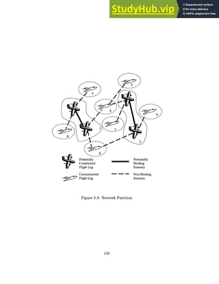
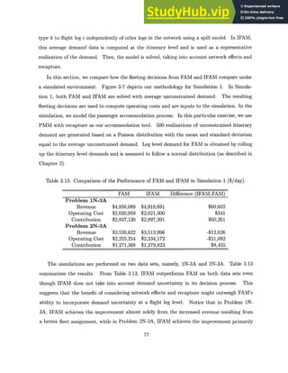
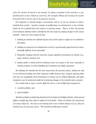
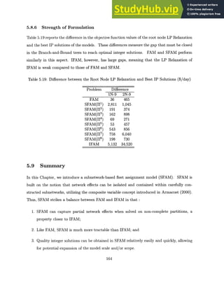
Table 5.14: Runtimes (sec) for Data Set 1N-9
Problem Preprocess Non-Parsimonious Parsimonious
LP Relax IP Total LP Relax IP Total
FAM 0 97 893 990 N/A N/A N/A
SFAM(HI
1 ) 6 99 397 502 103 419 528
SFAM(H 2
) 9 96 557 662 103 631 743
SFAM(1 3) 11 146 428 585 121 485 617
SFAM(H 4 ) 16 147 646 809 109 815 940
SFAM(H5
) 22 133 597 752 111 376 509
SFAM(1J6
) 285 N/A N/A N/A 153 1,495 1,933
SFAM(117
) 342 N/A N/A N/A 203 2,480 3,025
SFAM(H 8
) 1,007 N/A N/A N/A 249 1,187 2,443
IFAM 0 100 6,831 6,931 N/A N/A N/A
Table 5.15: Runtimes (sec) for Data Set 2N-9
Problem Preprocess Non-Parsimonious Parsimonious
LP Relax IP Total LP Relax IP Total
FAM 0 75 855 930 N/A N/A N/A
SFAM(H1) 5 81 772 858 74 753 832
SFAM(H 2
) 8 78 680 766 69 656 733
SFAM(1 3
) 12 87 775 878 78 723 813
SFAM(]J 4) 25 115 747 887 96 453 574
SFAM(11 5
) 35 342 1,156 1,533 98 396 529
SFAM(r16
) 795 N/A N/A N/A 280 4,954 6,029
SFAM(11 7
) 902 N/A N/A N/A 299 4,862 6,063
SFAM(11 8) 1542 N/A N/A N/A 348 5,093 6,983
IFAM 0 194 285,955 286,149 N/A N/A N/A
160

to fractionality problem.
5.8.4 Contribution
Table 5.16: Contributions ($/day) for Data Set 1N-9
Problem Estimated Actual
Revenue Opt. Cost Contr. Revenue Opt. Cost Contr.
FAM 35,317,041 13,915,419 21,401,622 35,094,234 13,915,419 21,178,815
SFAM(1I) 35,222,239 13,858,726 21,363,513 35,085,948 13,858,726 21,227,222
SFAM(l 2
) 35,190,844 13,858,205 21,332,639 35,085,948 13,858,205 21,227,743
SFAM(11 3
) 35,195,333 13,863,706 21,331,627 35,092,701 13,863,706 21,228,995
SFAM(H 4) 35,194,359 13,863555 21,330,804 65,092,701 13,863,555 21,229,146
SFAM( 5
) 35194,222 13863,724 21,330,498 35,092,883 13,863,724 21,229,159
SFAM(116
) 35,180,457 13,863,539 21,316,918 35,092,867 13,863,539 21,229,148
SFAM(11 7
) 35,180,616 13,863,813 21,316,803 35,092,869 13,863,813 21,229,056
SFAM(118
) 35,180,405 13,863,640 21,316,765 35,092,687 13,863,640 21,229,047
IFAM 35,092,750 13,865,244 21,227,506 35,092,750 13,865,244 21,227,506
Tables 5.16 and 5.17 summarize the
sented in Section 5.5 as a minimization
maximized contributions. Two sets o
contributions using SFAM.
model, but Tables 5.16 and
Notice that SFAM is pre-
5.17 report the equivalent
f numbers are reported, estimated and actual. The
estimated numbers are the numbers reported by the models (FAM, SFAM, and IFAM). Recall
that FAM and SFAM (when SFAM is not solved on complete partitions) use estimated spill
cost. The actual numbers are the revenues corresponding to a consistent, optimal passenger
mix. For IFAM, both sets of numbers are the same because IFAM always maintains consistent
passenger flows. The difference between the estimated contribution and the actual contribution
measures the cross-network error (erls) explained in Section 5.7. These differences are reported
in Table 5.18.
In Data Set 1N-9, the estimated contributions decrease monotonically as we move from FAM
to IFAM, as expected (recall discussion in Section 5.7). The actual contributions of SFAM see
significant improvement from FAM at approximately $50,000 daily or $18.4 million annually
(assuming a repeating 365-day calender). Notice that IFAM, interestingly, produces solution
that is inferior to most SFAM solutions. This could be the result of fractionality problem
in IFAM, resulting in longer solution time and wider optimality gap, the difference between
161

the best integer solution and the LP relaxation bound. Specifically, the optimality gap of
IFAM in this problem is $2,644, while the optimality gaps of SFAM and FAM are virtually nil.
Furthermore, IFAM optimality gap presents a proof that SFAM, in fact, has achieved optimal
fleeting for the problem because the upper bound on the contribution of IFAM, which is the
true upper bound, is $21,230,150, while the best contribution from SFAM is $21,229,159-a $991
difference. Note that in these exercises, we do not consider recapture.
In Data Set 2N-9, again, the estimated contributions form a monotonically decreasing trend
as expected. The actual contributions of SFAM on smaller partitions, interestingly, are inferior
to those of FAM. This can happen, as explained in Section 5.7 and illustrated in Figure 5-9.
The improvements over FAM are achieved when we solve SFAM on larger partitions. The
improvements are approximately at $1,100 daily or $405,000 annually. The IFAM optimality
gap is $9,641, which is much larger than those for FAM or SFAM. Deriving from this gap,
the upper bound on the contribution of this problem is therefore $24,862,350. SFAM achieves
a best solution of $24,855,936 on Partition H6. Thus, SFAM is $6,414 from the true upper
bound. Recall that the runtime of IFAM is more than 3 days on this problem and yet it could
not close the optimality gap. This shows that IFAM has a significant fractionality issue.
5.8.5 Actual Cross-Network Error
Tables 5.18 summarizes the actual cross-network errors (els) introduced in Section 5.7. We
can see that in both problems, the actual cross-network errors become smaller as we increase
the size of partitions. Notice also that the rate of decrease tapers off as we approach Partition
H8. This can be interpreted as implying that a boundary exists in terms of capturing network
effects. In order to break this boundary, we might need to construct significantly larger or
more consolidated partitions.
It is important to note that these actual cross-network errors do not necessarily relate
directly to the quality of the fleeting. Consider, for example, Data Set 1N-9. While the cross-
network error of SFAM(11 5
) is $13,621 larger than that of SFAM(H), the resulting fleeting of
SFAM(H 5
) is better than that of SFAM(118) (Table 5.16).
162

Table 5.17: Contributions ($/day) for Data Set 2N-9
Problem Estimated Actual
Revenue Opt. Cost Contr. Revenue Opt. Cost Contr.
FAM 38,334,548 13,326,430 25,008,118 38,181,255 13,326,430 24,854,825
SFAM(I 1 ) 38,302,209 13,325,197 24,977,012 38,178,997 13,325,197 24,853,800
SFAM(H2) 38,288,802 13,322,592 24,966,210 38,176,981 13,322,592 24,854,389
SFAM(H3) 38,283,478 13,324,452 24,959,026 38,179,218 13,324,452 24,854,766
SFAM(1 4) 38,269,436 13,334,415 24,935,021 38,189,591 13,334,415 24,855,176
SFAM(H5) 38,268,862 13,334,148 24,934,714 38,189,591 13,334,148 24,855,443
SFAM(H 6) 38,254,222 13,336,231 24,917,991 38,192,167 13,336,231 24,855,936
SFAM(H 7) 38,260,673 13,344,185 24,916,488 38,199,258 13,344,185 24,855,073
SFAM(1 8) 38,252,249 13,336,233 24,916,016 38,192,167 13,336,233 24,855,934
IFAM 38,209,998 13,357,289 24,852,709 38,209,998 13,357,289 24,852,709
Table 5.18: Actual Cross-Network Errors ($/day) for Data Set 1N-9
Problem Actual Cross-Network Errors
1N-9 2N-9
FAM 222,807 153,293
SFAM(H 1 ) 136,291 123,212
SFAM(11 2
) 104,896 111,821
SFAM(11 3
) 102,632 104,260
SFAM(114) 101,658 79,845
SFAM(115 ) 101,339 79,271
SFAM(H6 ) 87,770 62,055
SFAM(117 ) 87,747 61,415
SFAM(118 ) 87,718 60,082
IFAM N/A N/A
163

5.8.6 Strength of Formulation
Table 5.19 reports the difference in the objective function values of the root node LP Relaxation
and the best IP solutions of the models. These differences measure the gap that must be closed
in the Branch-and-Bound trees to reach optimal integer solutions. FAM and SFAM perform
similarly in this aspect. IFAM, however, has large gaps, meaning that the LP Relaxation of
IFAM is weak compared to those of FAM and SFAM.
Table 5.19: Difference between the Root Node LP Relaxation and Best IP Solutions ($/day)
Problem Difference
1N-9 2N-9
FAM 36 465
SFAM(1I1) 2,811 1,045
SFAM(H 2
) 191 374
SFAM(1 3
) 162 898
SFAM(H 4) 69 271
SFAM(H 5) 53 457
SFAM(H6 ) 543 856
SFAM(11 7) 758 6,040
SFAM(H 8) 198 730
IFAM 5,132 34,520
5.9 Summary
In this Chapter, we introduce a subnetwork-based fleet assignment model (SFAM). SFAM is
built on the notion that network effects can be isolated and contained within carefully con-
structed subnetworks, utilizing the composite variable concept introduced in Armacost (2000).
Thus, SFAM strikes a balance between FAM and IFAM in that :
1. SFAM can capture partial network effects when solved on non-complete partitions, a
property closer to IFAM;
2. Like FAM, SFAM is much more tractable than IFAM; and
3. Quality integer solutions can be obtained in SFAM relatively easily and quickly, allowing
for potential expansion of the model scale and/or scope.
164

We address two primary challenges, partition construction and column enumeration, and
successfully implement the prototype model for SFAM. We demonstrate the capability of SFAM
by testing it on full-size U.S. domestic schedules of a major U.S. airline. Preliminary results
suggest that SFAM is capable of producing better fleet assignments than FAM in comparable
time. IFAM, on the other hand, suffers significant fractionality issue, which is carried over
when we extend it to include schedule design, as shown in Chapter 4. The success of SFAM
crucially hinges on network partitioning, that is, how network effects are separated and handled.
Furthermore, notice that SFAM might require some experimentation with different network
partitionings in order to achieve optimal solution. In other words, it is not necessary that finer
partitioning would always yield better solution. We do not consider recapture in our current
implementation. Chapter 6 addresses recapture and other potential extensions.
165

Chapter 6
Subnetwork-Based Fleet Assignment
Model Extensions
6.1 Introduction
In Chapter 5, we introduce the subnetwork-based fleet assignment (SFAM). We show that
SFAM can sufficiently capture network effects, producing a fleet assignment equivalent to IFAM
in much less time. We have not, however, considered the recapture process, another important
element in the fleeting process. Recall that recapture is the phenomenon in which passengers
are re-accommodated on itineraries other than their desired itineraries. In this chapter, we
present two approaches for incorporating recapture into the fleeting process.
Recall from Chapter 5 that one of the main objectives of SFAM is to provide a kernel model
that can be extended to address other aspects of the planning process. In this chapter, we
discuss an alternate approach to the integration of schedule design and fleet assignment process
using SFAM.
6.1.1 Outline
In Section 6.2, we discuss how we can extend SFAM in a straightforward manner to allow for
recapture. An alternate approach for incorporating recapture is discussed in Section 6.3. We
discuss, in Section 6.4, how we might employ the subnetwork-based fleet assignment model in
167

the context of the schedule design problem discussed in Chapter 4.
6.2 SFAM with Recapture
In this section, we show how SFAM can be extended in a rather straightforward manner to
incorporate recapture. We describe the algorithm and state the potential difficulties. An
alternative approach that could bypass such difficulties is explained in the next section.
Recall that IFAM and SFAM capture network effects by ensuring consistent passenger flow,
that is, once passengers are spilled from one leg in a itinerary, they are spilled on all legs
contained in the itinerary. In addition, IFAM is able to model the recapture process, in which
some proportion of the otherwise spilled passengers are re-accommodated, or recaptured, on
alternate itineraries. Recall that IFAM models the recapture process utilizing traffic variables
(tr) and recapture rates (bp). Specifically, a number (tr) of passengers desiring itinerary p will
be redirected to alternate itinerary r, in the event that itinerary p contains at least one flight
that is capacitated. Only a proportion of these passengers, however, will accept itinerary r.
This proportion is bp, the recapture rate from p onto r. Thus, t'br is the number of passengers
desiring itinerary p who are successfully redirected to itinerary r. In this section, we show how
we can model recapture in SFAM in a similar fashion.
6.2.1 Modeling Recapture in SFAM
We show in Chapter 5 how we can partition a network into several independent and spill-
contained subnetworks. Spills in these subnetworks do not interact with one another. Hence,
within each subnetwork, all interactions among member flight legs including recapture can be
captured fully. To understand why, recall from Section 5.4 that for each fleet assignment
to member flight legs, a consistent, revenue-maximizing passenger flow can be determined.
Although in Chapter 5, we do not consider recapture, it can be modeled within each subnetwork
by simply allowing recapture of spilled passengers on alternate itineraries within the subnetwork.
This can be accomplished easily using the Passenger Mix Model (PMM) reviewed in Chapter
3. Specifically, for each fleet assignment to a subnetwork of flights, PMM is used to maximize
revenue, allowing recapture of spilled passengers within the subnetwork. This is possible only
168

8:00 AM
- A B
10:00 AM|
B - C
10:00 AM
-- A--
-B 2
12:00 PM
B-C
Figure 6-1: An Example of Network Partition that Does Not Allow Effective Modeling of
Recapture
when there exist alternative itineraries within the same subnetwork to which passengers can
be redirected. Partitions constructed using the algorithm described in Chapter 5, however, do
not necessarily provide such opportunities.
Consider, for example, a sufficiently complete partition constructed from the algorithm
described in Chapter 5, depicted in Figure 6-1. Suppose that Subnetwork 1 includes 2 flight legs,
one covering cities A-B, departing A at 8:00 AM, and the other covering cities B-C, departing
B at 10:00 AM. Subnetwork 2 cover similar flight legs but at different times; in particular,
A-B departs at 10:00 AM and B-C departs at 12:00 PM. In other words, Subnetworks 1 and
2 cover the same markets but at different times of day, therefore, recapture can occur between
Subnetworks 1 and 2. The network partition depicted in Figure 6-1 allows network effects
without recapture to be modeled fully, but is not adequate to model the effects of recapture.
Thus, our subnetwork generation procedure must be modified to ensure effective consideration
of recapture. In Figure 6-1, for example, Subnetworks 1 and 2 must be combined into one to
allow for recapture.
169

6.2.2 Building Network Partitions for SFAM with Recapture
We discuss how to partition the network to allow for recapture. All notation used is similar to
that described in Sections 5.3 and 5.5, with one exception. In order to distinguish SFAM with
recapture from its counterpart, SFAM without recapture, we include a subscript r to all notation
associated with the Subnetwork-Based Fleet Assignment Model with Recapture (SFAMr). For
example, H denotes a Partition S allowing for recapture, while H'S represents Partition S with
recapture ignored.
Full and Complete Partitions for SFAM with Recapture
On the full partition, HI, in which all flight legs are contained in one subnetwork, SFAMr
can model both network effects and recapture using the PMM model with recapture. Thus,
solving SFAMr on the full partition yields an optimal solution equivalent to that of IFAM with
recapture. (Recall that IFAM is the integration of FAM and PMM.) As in SFAM, however,
it is impractical if not impossible to solve SFAMr on the full partition for a full-size problem,
typically containing 2,000 flight legs and 10 fleet types.
We define the complete partition, HC, for SFAM with recapture as a partition in which all
network effects and recapture can be modeled fully. Thus, by definition, Hf is a complete
partition; there might exist, however, complete partitions with more independent subnetworks
than in HTF.
Sufficiently Complete Partitions for SFAM with Recapture
Similar to SFAM, there might exist a sufficiently complete partition IT6C, considering all network
effects and recapture, with the number of subnetworks, MAC, far greater than in HF (that is,
Mrc >> Mf). Notice that HIc can be (and often is) different from 1SC. To see why,
consider Figure 6-1, which depicts ISC for the sample network. ITSc for this network would
contain a total of 5 subnetworks, with Subnetworks 1 and 2 shown merged into one subnetwork.
Constructing the sufficiently complete partition for SFAMT is more involved than that for
SFAM. To do so, we begin by constructing the sufficiently complete partition ITSC, ignoring
possible recapture. Next, for each potentially constrained leg i, we identify markets that it
serves. We assume, as in IFAM, that recapture can occur only within the same market. Next,
170

for each identified market that i serves, we go through the list of itineraries in that market and
exclude those that contain i. The remaining itineraries are referred to as alternate itineraries.
We connect the flight legs included in these alternate itineraries to the subnetwork containing
i. The rational for including these itineraries in i's subnetwork is that possible recapture can
occur on these itineraries if flight leg i becomes constrained and passengers are redirected off
,t.
We repeat this procedure for every potentially constrained legs in the network. The final
result is the sufficiently complete partition HSC allowing fully for recapture. Solving SFAM,
on HSC is equivalent to solving SFAMr on H" yielding an optimal solution equivalent to that
of IFAM with recapture.
Notice that HISc might be highly consolidated due to the connectivity resulting from flight
leg interdependencies and recapture. Thus, a challenge is to partition the network such that
network effects and recapture can be modeled both sufficiently and efficiently.
Constructing Tractable Partitions for SFAM with Recapture
We propose a two-step heuristic approach for constructing tractable partitions for SFAM with
recapture.
STEP 1. Construct the sufficiently complete partition HSC ignoring possible recapture, and
subdivide this partition into a pre-specified size using one of the procedures described in Section
5.6.
STEP 2. For each potentially constrained leg i, identify its candidate markets. Candidate
markets for i are markets with a high potential of being spilled from leg i, such as, markets with
lower fares or with extra capacity elsewhere. For each of the candidate markets, we identify
candidate alternateitinerarieswithin the market. The candidate alternate itineraries, a subset
of all alternate itineraries, are those with high recapture rates for spill from i and with excess
capacity. We connect only those legs contained in the candidate alternate itineraries to the
subnetwork containing i.
Repeat STEP 2 for all potentially constrained legs.
171

This algorithm is not guaranteed to produces effective partitions. It sacrifices the exactness
of a sufficiently complete partition for the tractability of smaller subnetworks. If the resulting
partition from STEP 2 is too large, this process is repeated using smaller pre-specified size
limits in STEP 1, and/or limiting the number of candidate markets and alternate itineraries
considered in STEP 2.
6.2.3 SFAM with Recapture: Formulation and Solution Algorithm
M, 9
Min E (C S)(fis) (6.1)
m=1 n=1
Subject to:
My ?7
SZ(6 ) (fs) 1 ,Vi E L (6.2)
m=1 n=1
My U
Yk,o,t- + K
> Z(a)(f s)
iEI(k,o,t) m=1 n=1
My ?S
yk,o,t+ - S S S( s)k (fs) = 0 ,Vk,o,t E N (6.3)
iEO(k,o,t)m=1 n=1
MU
YkOtm + S) <_ Nk ,Vk E K (6.4)
oEA iECL(k) m=1 n=1
(f ) C {0, 1} ,Vn E Fr~s, Vm E II (6.5)
Yk,o,t ;> 0 ,V{k, o, t} c N (6.6)
No modification to the structure of the SFAM model presented in Section 5.5 is necessary in
modeling recapture. Only the objective function coefficients of the assignment variables need
to be altered. Recall that (C7js) is the assignment cost when there is no recapture of instance
n, subnetwork m, and partition IS in a minimization model of SFAM. (Note that (Cm )n can
equivalently represent the estimated contribution in a maximization model of SFAM.) Thus,
in SFAM,, we use (Cm ) to denote the assignment cost when there is recapture of instance
rpa
n, subnetwork m, and partition 1 1 S in a minimization model of SEAM. In particular, this
172

assignment cost includes operating costs, passenger related costs, and net spill costs (after
recapture).
Reiterating, apart from the fact that network partitions are constructed differently for
SFAM., the only difference to the formulation is in the objective function coefficient. Thus, the
same solution algorithm used for SFAM in Section 5.6 can be applied to SFAMr-
In this section, we describe in detail an approach for considering recapture, using the
subnetwork-based fleet assignment model (SFAMr). The major challenge lies in construct-
ing tractable partitions that sufficiently modeling both network effects and recapture. Given a
partition, recapture effects within each subnetwork can be assessed using PMM with recapture
(reviewed in Chapter 3). While there can be errors associated with not modeling possible
recapture between subnetworks, we hypothesize that these errors will not significantly affect
the quality of the fleeting, as evidenced in Chapter 5. Because the success of SFAM, depends
on the construction of tractable, yet sufficiently connected, partitions and it is yet to be shown
that the proposed algorithm produces such partitions, we consider an alternate approach for
modeling recapture in the fleeting process.
6.3 An Alternate Modeling Approach for Recapture
In this section, we describe an alternate approach for modeling recapture in the fleeting process.
The key idea is to consider recapture external to the fleeting process, and solve the fleet as-
signment model without recapture. The motivation is to achieve greater tractability in the
fleeting process, while attempting to incorporate recapture. This algorithm relies on an effective
demand adjustment module, whose specification requires further research.
Figure 6-2 depicts a conceptual flow diagram of our proposed approach. This approach is
iterative and is comprised of three distinct modules:
1. the fleeting module,
2. a passenger allocation module, and
3. a demand adjustment module.
173

START
i =0;
*FFleeting (i);I
Pax (i);
Adjust Demand
Pattern;
i
Has the
NO Stopping
Criteria
been met?
YES
STOP
Figure 6-2: A Conceptual Diagram for Modeling Recapture Externally in the Fleeting Process
174

The fleeting module optimizes the fleeting of the schedule based on demand inputs at that
iteration, ignoring recapture. FAM, SFAM or IFAM without recapture can be used in the
fleeting module. We denote the iteration i fleeting as Fleeting(i). The passenger alloca-
tion module assigns passengers to itineraries based on Fleeting(i), the input demands, and
recapture rates. PMM with recapture can be applied in the passenger allocation module. We
denote the resulting passenger mix at iteration i as Pax(i).
The demand adjustment module analyzes Pax(i) and suggests alternate input demands,
with the idea of generating a better fleeting in the next iteration.
The algorithm starts with the iteration index, i, set to zero. A fleet assignment model
is solved based on initial demands to obtain Fleeting(i). Next, passenger flow Pax(i) is
determined based on Fleeting(i) and initial demands. Note that associated with Pax(i)
is an estimate of contribution of Fleeting(i). If i = 0, the stopping criteria is ignored
and the algorithm continues on the "NO" branch. The demand adjustment module analyzes
Pax(i), looking in particular for potential recapture opportunities. Adjusted input demands
are generated taking into account potential recapture opportunities and the iteration counter
is increased. The subsequent iteration begins by solving a fleet assignment model using the
adjusted demand inputs, resulting in Fleeting(i+1). Pax(i+1) is then determined based on
Fleeting(i+1) and the initial demands. The contribution of Fleeting(1) is estimated based
on Pax(1). The following stopping criteria can be used:
1. if a pre-specified improvement over Fleeting(O) is achieved, or
2. if i exceeds some pre-specified iteration count.
The first criterion compares the contribution of Fleeting(1) and Fleeting(O). If the
improvement exceeds a pre-specified goal, the algorithm stops. The fleeting of the last iteration
is the selected fleeting. If the improvement does not exceed the pre-specified goal, the algorithm
continues on the "NO" branch. There might be instances, however, in which the pre-specified
goal cannot be achieved, in which case, the algorithm stops after a pre-specified number of
iterations and the fleeting from the iteration that yields the highest contribution is the selected
fleeting.
175

6.4 SFAM in the Context of Schedule Design
Recall that in Chapter 4, we present the Integrated Schedule Design and Fleet Assignment
Model with Constant Market Share (ISD-FAM). The key underlying idea of ISD-FAM is
to use recapture rates to reallocate passengers in the event that flight legs are deleted from
the schedule. Although ISD-FAM is more tractable than its counterpart, ISD-FAM, it still
suffers from serious fractionality issues, inherited from IFAM. In this section, we discuss a new
approach to the schedule design problem based on SFAM. We anticipate that the strength of
the SFAM LP relaxation allow greater solvability.
6.4.1 The Schedule Design Problem with Constant Market Share
We can alternatively formulate ISD-FAM using SFAM, as the core, as follows:
ins
M1-1s
Min E (Cs) (fYs)
m=1 n=1
(6.7)
Subject to:
M ns
(ogs)i (ns)
m1 n=1
r nnr
m=1 n=1
MM
Yo
E +
k m 5 (,rn)k i=)
r nns
-yk,o,t± - (
> 5 g )k (fn)
iEO(k,o,t) m=1 n=1
Sns
Yk,o,tm + (SIs (-Is
oEA iCL(k) m=1 n=1
(fb
s)
ymot
= 1 ,Vi E LF
< 1 ,Vi E LO
= 0 ,Vk,o,t E N
< Nk ,Vk E K
E {0, 1} ,Vn E Frms Vm E IIc
> 0 ,V{k,o,t} E N
176
(6.8)
(6.9)
(6.10)
(6.11)
(6.12)
(6.13)

To understand the applicability of SFAM, to the schedule design problem, consider the
notion of a zero-seatfleet type. Notice that a decision to delete an optional flight leg i from the
schedule is equivalent to a decision to fleet a fictitious fleet type of capacity zero to flight leg i.
Thus, the schedule design problem can be thought of as a special fleet assignment problem with
a special zero-seat fleet type available (only) to all optional flight legs. In building network
partitions, all optional flight legs are then, by definition, potentially constrained legs.
Because of the zero-seat fleet type, the connectivity of the subnetworks becomes even
stronger than in usual instances of SFAMr. Specifically, the sufficiently complete partition
IS'C of SFAMr in the presence of zero-seat fleet types, is more consolidated. Moreover, the
construction of tractable yet sufficiently connected partitions becomes more challenging. Thus,
the alternate approach for modeling recapture described in Section 6.3, might be more viable.
Apart from reduced complexity, there is an added benefit to using the approach depicted in
Figure 6-2. By employing the demand adjustment module externally, we might be able to
capture demand and supply interactions arising from deletion of flight legs with each iteration
of the loop in Figure 6-2.
177

Chapter 7
Conclusions
In this chapter, we summarize findings and contributions of this dissertation and provide direc-
tions for future research.
7.1 Summary of Contributions
In Chapter 1, we present an extended overview of the airline planning process, discussing the
tasks and importance of each step and providing references to relevant literature. A detailed
description of one airline's planning process is provided. Throughout the rest of the dissertation,
we discuss in detail the problems of airline fleet assignment and schedule design. We summarize
our findings and contributions in the contexts of these two problems.
7.1.1 Fleet Assignment
In Chapter 3, we show that significant benefits, as large as $100 million per year, are achievable
by incorporating network effects and recapture in fleeting models. The benefit of recapture,
however, depends largely on the opportunities for recapturing. Opportunities for successfully
recapturing diminish as capacity on alternate itineraries becomes more fully assigned. Recap-
ture also yields less benefit when the network is fairly under-utilized because there are fewer
spilled passengers, resulting in fewer recaptured demands.
Our experiments show that in IFAM, fleeting decisions are not particularly sensitive to
a range of recapture rates. Specifically, IFAM produces relatively consistent fleetings over
179

this limited range. We show through simulations that although IFAM takes as input average
demand ignoring uncertainty (unlike FAM), the ability to account for network effects allows
IFAM to produce better assignments than FAM. This clearly suggests that capturing flight
leg interdependence is more important than capturing demand uncertainty in hub-and-spoke
network fleet assignment problems. In addition, we show that the optimal passenger mix
assumption in IFAM is acceptable and is not too limited. Specifically, although contributions
of both FAM and IFAM in our simulation are less than the corresponding contributions when
optimal passenger mix is assumed, IFAM still produces better assignments than does FAM. We
also show that both FAM and IFAM are sensitive to demand forecast errors, but no significant
trends can be established as to which model is more robust in handling such errors. There is
some evidence, however, suggesting that IFAM's fleeting is less sensitive to forecast errors with
overestimated demands than with underestimated demands.
In Chapter 5, we revisit the issue of network effects in fleeting and introduce the subnetwork-
based fleet assignment model (SFAM). SFAM is built on the notion that network effects can
be isolated and contained within carefully constructed subnetworks, utilizing the composite
variable concept introduced in Armacost (2000). Thus, SFAM strikes a balance between FAM
and IFAM in that :
1. SFAM can capture (partial) network effects when solved on (non-complete) partitions,
like IFAM;
2. Like FAM, SFAM is much more tractable than IFAM; and
3. Quality integer solutions can be obtained in SFAM relatively easily and quickly, allowing
for potential expansion of the model scale and/or scope.
We address two primary challenges, partition construction and column enumeration, and
successfully implement the prototype model for SFAM. We demonstrate the capability of SFAM
by testing it on full-size U.S. domestic schedules of a major U.S. airline. Preliminary results
suggest that SFAM is capable of producing better fleet assignments than FAM, in comparable
time. The success of SFAM crucially hinges on network partitioning, that is, how network
effects are separated and handled. A critical advantage of SFAM is its potential to integrate
further airline planning problems, namely, schedule design and fleet assignment.
180

In Chapter 6, we discuss some potential extensions of SFAM. We provide a detailed discus-
sion of how recapture can be modeled in SFAM. The subnetwork-based fleet assignment model
with recapture (SFAMr) is introduced. The major algorithmic challenge lies in constructing
tractable partitions that allow for effective modeling of both network effects and recapture. We
describe an algorithm for constructing partitions in which recapture can be modeled. We re-
visit the modeling approach for recapture used in IFAM and SFAM, and introduce an approach
that makes recapture external to the fleeting process. We then provide a high level description
of a potential algorithm to achieve this.
7.1.2 Schedule Design
In Chapter 4, we review the concept of demand and supply interaction. Integration of the
fleeting and schedule design processes is accomplished by extending IFAM. Our approach to
the schedule design problem is incremental, in that modifications are made to a base schedule.
We describe an approach for constructing a master flight list, which includes mandatory and
optional flights. Two models are developed, based on variable market share, and constant
market share assumptions.
In the integrated schedule design and fleet assignment model with constant market share
(ISD-FAM), we assume that the market share of the airline remains constant with schedule
changes. ISD-FAM utilizes a recapture mechanism to re-accommodate passengers when flight
legs are deleted from the schedule. Although market share is assumed to be constant, some
interactions between demand and supply can be captured indirectly. While the constant market
share assumption might not be accurate under all scenarios, we demonstrate its applicability.
We investigate its performance and report computational results.
In the extended schedule design and fleet assignment model (ESD-FAM) , the market share
of the airline changes with schedule changes. We describe in detail our approach for the
treatment of demand and supply interactions, utilizing demand correction terms. We present
model formulations, solution algorithms, and computational experiences. Our experiments
show that ESD-FAM has a weak LP relaxation, similar to IFAM. Demand correction terms
adversely affect the solvability of the model further.
In Chapter 6, we provide a high level description of how the subnetwork-based fleet assign-
181

ment model might be applicable to the schedule design problem. We introduce the notion of
a zero-seat fleet type, which enables us to view the schedule design problem as a special fleet
assignment problem. Hence, the applicability of SFAM with recapture to the schedule design
problem follows directly. We believe that the approach for modeling recapture introduced in
Section 6.3 might be more viable, conditioned upon the effectiveness of its demand adjustment
module. By employing the demand adjustment module externally, we can significantly simplify
the subnetwork construction process because of limited network connectivity. In addition, we
might be able to capture the demand and supply interactions using the demand adjustment
module as we iterate in the solution process.
7.2 Directions for Future Research
7.2.1 Integrated Schedule Design and Fleet Assignment
As with any modeling, a number of assumptions are made in our efforts to tackle the schedule
design and fleet assignment problems. Some of these assumptions are necessary to simplify
the problem and increase tractability, while others are made to facilitate operation policies.
Sometimes these assumptions are difficult to justify; they are necessary, however, in order to
allow efficient tackling of the problems at hand. Future research should see some relaxation of
these assumptions. If full relaxation is infeasible, measures to validate included assumptions
are needed.
A significant assumption that must be tested is the absence of competitors' interactions.
Although we allow for changes in market shares in our schedule design models, we do not at-
tempt to model direct competitors' reactions to our schedule modifications. This is particularly
significant if the changes recommended are to increase the frequency. Our models, in their
current forms, assume that competitors will operate at the same frequency as before. This
is highly unlikely, however, given the level of competition observed in the industry. Should
the competitors decide to match our offerings, the forecasted demands could be significantly
overestimated.
Demand and supply interaction issues in the schedule design problem represent a major
research area that is yet to be fully investigated, understood, and modeled. With better
182

understanding of these interactions, efficient modelling techniques can be developed to tackle
the schedule design problem. Competitors' reactions could also be modeled in the form of
demand and supply interactions.
Notice as well that the current forms of our integrated models for schedule design and
fleet assignment ignore a number of operational issues. These issues include, for example,
maintenance of hub structure, airline presence in markets, minimum or maximum frequency in
markets, gate and slots availability, etc. Thus, an operational model requires addition of these
considerations to ensure an appropriate schedule.
7.2.2 Multiple Fare Class Models
In Chapter 3, we quantify the benefit of network effects and recapture using fare-class aggregated
demand. Further studies should be commissioned to investigate the benefits of modeling
multiple fare classes in the fleeting process. In order to benefit fully from the fare class
level model, however, the actual fleeting and revenue management processes must be closely
coordinated.
A theoretical framework exists to model multiple fare classes in the fleet assignment model
(see Kniker, 1998, for example). No attempts have been made, however, to measure the
potential benefits. This is in part because good quality fare-class level forecasts are difficult to
obtain well in advance of the departure date. Thus, data availability is another major hurdle
that must be overcome.
Another important issue that might have to be addressed is the deterministic demand
assumption. At itinerary, fare class level, demand is highly volatile, assuming deterministic
demand might no longer be justifiable.
7.2.3 Subnetwork Based Fleet Assignment
The primary motivation for the subnetwok-based fleet assignment model (SFAM) is for it to be
a kernel for further integrated schedule planning models. We show in Chapter 5 that SFAM
can solve fleet assignment problems relatively efficiently. In Chapter 6, we discuss at length
two ways to include recapture in SFAM. Based on that, we propose an approach to apply
SFAM to the schedule design problem. There are many other potential extensions to SFAM
183

as discussed below.
A Subnetwork-Based Fleet Assignment Model with Time Windows
The fleet assignment with time windows model by Rexing, et al (2000) extends the leg-based
fleet assignment model by allowing minor re-timings of flight legs in order to provide greater
opportunities to increase aircraft utilization. (We review their model in Chapter 2.) Like
any leg-based model, their model does not consider network effects or recapture. Thus, SFAM
could be expanded to produce a subnetwork-based fleet assignment model with time windows,
considering network effects, recapture and re-timing of flight legs.
A Subnetwork-Based Fleet Assignment Model with Stochastic Demand
A major assumption in IFAM is the deterministic demand assumption. Although we show
in Chapter 3 that even with this assumption, IFAM is able to produce better assignments
than FAM because IFAM accounts for network effects, the fact that IFAM does not consider
demand uncertainty leaves room for improvement. To further extend IFAM, however, seems
impractical because its increased complexity over FAM. SFAM might be a good candidate
for this extension. In fact, SFAM's approach to compute estimated contribution or spill cost
externally, that is, not as a part of model decision, allows convenient incorporation of stochastic
demand.
There are two elements that have to be addressed in SFAM with stochastic demand:
1. partition construction, and
2. spill cost calculation.
The partition construction algorithm has to be modified slightly to recognize the fact that
demand is stochastic. In particular, the definition of a potentially constrained leg has to
be modified. Previously, a potentially constrained leg is defined as a flight leg that has un-
constrained (deterministic) demand exceeding the capacity of the smallest fleet type. In the
stochastic case, we can aggregate itinerary demand at the flight leg level and assume that
leg-level demand follows a normal distribution (a common industry practice). A potentially
constrained leg can then be defined as a leg that has some probability, exceeding a pre-specified
184

threshold value, of having leg-level demand exceeding the capacity of the smallest fleet type.
This probability can be derived from the leg-level demand distribution. Once a flight is clas-
sified as a potentially constrained leg, it will be included in the partition construction process,
which could follow the same procedure described in Section 5.6.
Next, recall that associated with any instance of assignment of each subnetwork is an es-
timate of contribution or assignment cost, a part of which is the estimated revenue. In our
implementation, we assume a deterministic revenue-maximizing passenger configuration. We
can, alternatively, use other methods that account for the stochasticity in demand to estimate
this revenue. For example, FAM utilizes a spill model (see for example, Swan, 1979) to esti-
mate the revenue based on a given demand distribution for each fleet-flight assignment. For
multiple-flight subnetworks, new methods can be designed, possibly based on single-leg spill
models, to estimate the revenue based on given demand distributions. The estimated revenues
from these stochastic spill models can then be used in the objective function of SFAM, resulting
in a subnetwork-based fleet assignment model with stochastic demand.
7.3 Final Thoughts
This dissertation focuses on the two steps of the airline planning process, referred to as, sched-
ule design and fleet assignment. Although fleet assignment is a well-studied area, room for
improvements still exist. We develop models and algorithms that allow further integration
of the planning process. As we move toward greater integration, the scale and complexity of
the models grow rapidly, as illustrated in the integrated schedule design and fleet assignment
problem. We demonstrate through a number of experiments the applicability of our models
to actual problems faced by major airlines. Although some models might take long time to
achieve a solution, it should be noted that runtime is not always critical. Planners currently
take weeks to produce a schedule; thus, spending hours or days running a model that produces
improved schedules is clearly beneficial.
As we move forward, further integration of systems is clearly the preferred path, producing
improved, globally optimal airline solutions. The ultimate system is one in which all steps of
the planning process are optimized simultaneously. This system, however, is currently out of
185

reach, not only because of today's computational technology limitations but also the lack of
complete understanding of interactions among pieces.
186

Bibliography
J. Abara, "Applying integer linear programming to the fleet assignment problem," Interfaces
19 (1989).
R.K. Ahuja, T.L. Magnanti and J.B. Orlin, Network Flows: Theory, Algorithms, and Ap-
plications,Prentice-Hall, Inc (1993).
C. Barnhart, N.L. Boland, L. W. Clarke, R.G. Shenoi, "Flight String Models for Aircraft
Fleeting and Routing," TransportationScience, Vol. 32, No. 3, pp. 208-220.(1998).
C. Barnhart, A. Farahat, M. Lohatepanont, "Airline Fleet Assignment: An Alternative
Model and Algorithm," Working Paper, Massachusetts Institute of Technology, Cambridge,
MA (2001).
C. Barnhart, L. Hatay, and E.L. Johnson, "Deadhead Selection for the Long-Haul Crew
Pairing Problem," OperationsResearch 43, pp. 491-498 (1995).
C. Barnhart, C.A. Hane, E.L. Johnson and G. Sigismondi, "A Column Generation and
Partitioning Approach for Multi-Commodity Flow Problem," Telecommunication Systems, vol.
3., pp. 239-258 (1995).
C. Barnhart, T. Kniker, and M. Lohatepanont, "Itinerary-Based Airline Fleet Assignment,"
TransportationScience, To Appear (2001).
C. Barnhart, E. L. Johnson, G.L. Nemhauser, M.W.P. Savelsgergh and P.H. Vance, "Branch-
and-Price: Column Generation for Solving Huge Integer Programs," Report LEC-94-03, Geor-
gia Institute of Technology (1995).
C. Barnhart, K.T. Talluri, Chapter10: Airline OperationsResearch, Working paper (1996).
P. Belobaba, "Airline Yield Management: An Overview of Seat Inventory Control," Trans-
187

portationScience, Vol. 21, pp. 63-73 (1987).
P. Belobaba, "Application of a Probabilistic Decision Model to Airline Seat Inventory Con-
trol," OperationsResearch, Vol. 37, pp. 183-197 (1989).
P. Belobaba, "The Revenue Enhancement Potential of Airline Yield Management Systems,"
ASTAIR Proceedings: Advanced Software Technology for Air Transport, London, pp. 143-164
(1992a)
P. Belobaba, "Optimal vs. Heuristic Methods for Nested Seat Allocation," Presentation to
AGIFORS Reservations Control Study Group Meeting, Brussels, Belgium (1992b).
P. Belobaba, "Airline Planning Systems: Economics and Models," Lecture Note for 16.75
Airline Management, Massachusetts Institute of Technology (1999).
P. Belobaba, and A. Farkas, "Yield Management Impacts on Airline Spill Estimation,"
TransportationScience, Vol. 33, pp. 217-232 (1999).
M. Berge, "Timetable Optimization: Formulation, Solution Approaches, and Computational
Issues," AGIFORS proceeding, pp. 341-357 (1994).
D. Bertsimas and J. Tsitsiklis, Introductionto LinearOptimization,Athena Scientific (1997).
S. Bratu, "Network Value Concept in Airline Revenue Management," Master thesis, Massa-
chusetts Institute of Technology, Cambridge, MA (1998).
S. I. Brumelle, J. I. McGill, T. H. Oum, K. Sawaki, and M. W. Tretheway, "Allocation of
Airline Seats between Stochastically Dependent Demands," TransportationScience, Vol. 24,
pp. 183-192 (1990).
I. Buch, "Airport Ground Staff Scheduling at El Al," AGIFORS Proceeding, pp. 116-121
(1994).
Y. Chan, "Route Network Improvement in Air Transportation Schedule Planning," M.I.T.
Flight Transportation Laboratory, Report No. R72-3 (1972).
L. W. Clarke, E. L. Johnson, and G. L. Nemhauser, "Maintenance and Crew Considerations
in Fleet Assignment," TransportationScience, Vol. 30, pp. 249-260 (1996).
M. Clarke, "Development of Heuristic Procedures for Flight Rescheduling in the Aftermath
of Irregular Airline Operations," Sc.D. Dissertation, Massachusetts Institute of Technology,
Cambridge, MA (1997).
R. E. Curry, "Optimum Seat Allocation with Fare Classes Nested by Origins and Destina-
188

tions," TransportationScience, Vol. 24, pp. 193-204 (1990).
G. B. Dantzig and A. R. Ferguson, "The Problem of Routing - A mathematical Solution,"
Government Res. Report, Federal Clearinghouse, AD604395 (1954).
M.S. Daskin and N.D. Panayoyopoulos, "A Lagrangian relaxation approach to assigning
aircraft to routes in hub and spoke networks," TransportationScience, Vol. 23, pp.9 1
-9 9
(1989).
J. W. Devanney III, "Transportation Scheduling under Multi- Dimensional Demands" MIT
Department of Civil Engineering, Research Report R67- 72 (1967).
G. Dobson and P.J. Lederer, "Airline Scheduling and Routing in a Hub-and-Spoke System,"
TransportationScience, Vol. 27, pp. 281-297 (1993).
M.M. Etschmaier and D.F.X. Mathaisel, "Airline Scheduling: The State of the Art," AGI-
FORS proceeding, pp. 181-225 (1984).
M.M. Etschmaier and D.F.X. Mathaisel, "Airline Scheduling: An Overview," Transportation
Science, Vol. 19, pp. 127-138 (1985).
A. Farkas, "The Influence of Network Effects and Yield Management on Airline Fleet As-
signment Decisions," Doctoral Thesis, Massachusetts Institute of Technology, Cambridge, MA
(1996).
G. Gallego, "A Demand Model for Yield Management," Technical Report, Columbia Uni-
versity, Department of Industrial Engineering and Operations Research, New York, NY (1996).
G. Gallego and G. Van Ryzin, "A Multi-Produce Dynamic Pricing Problem and Its Appli-
cations to Network Yield Management," OperationsResearch, Vol 45, pp. 24-41 (1997).
J. Goodstein, "Re-Fleeting Applications at United Airlines," AGIFORS proceeding, pp.
75-88 (1997).
R. Gopalan and K. T. Talluri, "The Aircraft Maintenance Routing Problem," working paper
(1993).
C.A. Hane, C. Barnhart, E.L. Johnson, R.E. Marsten, G.L. Nemhauser and G. Sigismondi,
"The Fleet Assignment Problem: Solving a Large-Scale Integer Program," MathematicalPro-
gramming, vol. 70., pp. 211-232 (1995).
E. L'Heureux, "A New Twist in Forecasting: Short-Term Passenger Pickup," AGIFORS
proceeding, pp. 248-261, (1986).
T. Kniker, "Airline Itinerary-Based Fleet Assignment," Doctoral Thesis, Massachusetts
189

Institute of Technology, Cambridge, MA (1998).
T.L. Jacobs, B.C. Smith, and E.L. Johnson, "O&D FAM: Incorporating Passenger Flow
into the Fleeting Process," AGIFORS Presentation (1999).
E. Kambour, S. Sivaramakrishnan, and A. Boyd, "The Impact of O&D vs. Leg Forecasting
on the Demand Unconstraining Process," Presentation at INFORMS Fall 2000 Meeting, San
Antonio, TX (2000).
A.O. Lee, "Airline Reservations Forecasting: Probabilistic and Statistical Models of the
Booking Process," Ph.D. Thesis, Massachusetts Institute of Technology, Cambridge, MA (1990).
W. Lieberman, "The Integration of Pricing and Revenue Management," Presentation at
INFORMS Spring 2000 Meeting, Salt Lake City, UT (2000).
R.C. Lochan, "Long Haul Fleet Assignment: Models, Methods and Applications," Master
Thesis, Massachusetts Institute of Technology, Cambridge, MA (1995).
F. Lu, "Integrated Airline Scheduling: Models and Algorithms," Master Thesis, Massa-
chusetts Institute of Technology, Cambridge, MA (1997).
P. Marcotte, and G. Savard, "A Bi-Level Programming Model of Revenue Management in
the Airline Industry," Presentation at INFORMS Fall 2000 Meeting, San Antonio, TX (2000).
R. E. Marsten, R. Subramanian, L. Gibbons, "Junior Analyst Extraordinare (JANE),"
AGIFORS proceeding, pp. 247-259 (1996).
R.S. Mangoubi, D.F.X. Mathaisel, "Optimizing Gate Assignment at Airport Terminals,"
AGIFORS proceeding, pp. 419-450 (1984).
M. Nikulainen and K. Oy, "A Simple Mathematical Method to Define Demand for Schedule
Planning," AGIFORS proceeding, pp. 77-85 (1992).
U. Oppitz, and S. P6lt, "Unconstraining and Bid Pricing," AGIFORS proceeding, pp. 89-97
(1997).
T. H. Oum, A. Zhang, and Y. Zhang, "Inter-Firm Rivalry and Firm-Specific Price Elastici-
ties in Deregulated Airline Markets," Journalof TransportationEconomics and Policy, Vol 27.
pp. 171-192 (1993).
C.S. Papacostas and P.D. Prevedouros, TransportationEngineering and Planning, 2ed.,
Prentice-Hall, Inc (1993).
K.R. Rao, "A Methodology for Regional Bus Transit Network Planning," Ph.D. Thesis,
190

Indian Institute of Technology (1998).
B. Rexing, C. Barnhart, T. Kniker, and A. Jarrah, "Airline Fleet Assignment with Time
Windows," TransportationScience, vol 34, pp. 1-20 (2000).
A. Richardson, "Gate Manager," AGIFORS Proceeding, pp. 157-163 (1991).
R.G. Shenoi, "Integrated Airline Schedule Optimization: Models and Solutions Methods,"
Ph.D. Thesis, Massachusetts Institute of Technology (1996).
R.W. Simpson, "Computerized Schedule Construction for an Airline Transportation Sys-
tem," MIT Flight Transportation Laboratory report no. FT-66-3 (1966).
R.W. Simpson, "Scheduling and Routing Models for Airline Systems," MIT Flight Trans-
portation Laboratory report no. R68-3 (1969).
R.W. Simpson, "Using Network Flow Techniques to Find Shadow Prices for Market and
Seat Inventory Control," MIT Flight Transportation Laboratory Memorandum M89-1, MIT,
Cambridge, MA (1989).
R.W. Simpson, P.P. Belobaba, "The Demand for Air Transportation Services," Lecture
Note for 16.74 Air Transportation Economics, Massachusetts Institute of Technology (1992a).
R.W. Simpson, P.P. Belobaba, "The Supply of Scheduled Air Transportation Services,"
Lecture Note for 16.74 Air Transportation Economics, Massachusetts Institute of Technology
(1992b).
B.C. Smith, J.F. Leimkuhler, and R.M. Darrow, "Yield Management at American Airlines,"
Interfaces,Vol. 22, pp. 8-31 (1992).
F. Soumis, J.A. Ferland, and J.-M. Rousseau, "A Model for Large Scale Aircraft Routing
and Scheduling Problems," TransportationResearch, No. 14B, pp. 191-201 (1980).
R. Subramanian and R. Marsten, "A Unified Approach to Scheduling: Fleet Assignment
and Crew Planning," AGIFORS proceeding, pp. 311-319 (1994).
W. M. Swan, "A System Analysis of Scheduled Air Transportation Networks," Ph.D. Dis-
sertation, Massachusetts Institute of Technology, Cambridge, MA (1979).
D. Teodorovic, Airline OperationsResearch,Gordon And Breach Science Publishers (1989).
D. Teodorovic and E. Krcmar-Nozic, "Multicriteria Model to Determine Flight Frequencies
on an Airline Network under Competitive Conditions," TransportationScience, Vol. 23, pp.
14-25 (1989).
191

P.H. Vance, C.Barnhart, E.L. Johnson, and G.L. Nemhauser, "Airline Crew Scheduling: A
New Formulation and Decomposition Algorithm," OperationsResearch, Vol 45, No. 2, pp. 1-20
(2000).
J. Vanlaningham, and M. West, "Applications of OR and AI to Gate Scheduling: Or Two
Heads are Better Than One," AGIFORS Proceeding, pp. 229-241 (1988).
J.-L. Vaysse, "Airbus Industrie Fleet Planning," AGIFORS proceeding, pp. 27-43 (1998)
L. R. Weatherford, "Optimization of Joint Pricing and Allocation Perishable-Asset Revenue
Management Problems with Cross-Elasticity," Journalof CombinatorialOptimization, Vol 1.
pp. 277-304 (1997).
C.F. Wheeler, "Strategies for Maximizing the Profitability of Airline Hub-and-Spoke Net-
works," TransportationResearch Record, No. 1214, pp. 1-9 (1989).
E.L. Williamson, "Airline Network Seat Inventory Control: Methodologies and Revenue
Impacts," MIT Flight Transportation Laboratory Report R92-3, MIT, Cambridge, MA (1992).
S. White, "How to Win at Graphs and Influence People," AGIFORS Proceeding, pp. 305-
322, (1997).
R. D. Wollmer, "An Airline Seat Management Model for a Single-Leg Route When Low
Fare Classes Book First," OperationsResearch,Vol. 40, pp. 26-37 (1992).
S. Yan, and C. Tseng, "An Integrated Model and Solution Algorithm for Fleet Routing
and Flight Scheduling," Working Paper, National Central University, Chungli, Taiwan, ROC
(2000).
192

Appendix A
Glossary
aircraft day: a series of connecting flights that is flyable by a single aircraft in one day.
aircraft rotation: the sequence of flight legs that are flown by an aircraft beginning and
ending at the same station.
aircraft routing: the process which determines the actual aircraft rotation in a fleeted sched-
ule, the third step in the airline schedule planning process.
airline schedule planning process: the four-step sequential planning process consisting of
(1) schedule design, (2) fleet assignment, (3) aircraft routing, and (4) crew scheduling.
complete partition: a network partition in which network effects can be captured fully.
connecting bank or complex: a set of flights arriving or departing a hub airport in some
period of time..
crew pairing: a sequence of connected flight segments that begins at a crew base location,
and returns to the same location, within the maximum allowable time-away-from-base. A
pairing is a set of duty periods, separated by rest periods/overnightsthat satisfy all work
rules.
daily flight schedule: a flight schedule that repeats every day of the week.
deadhead: a flight leg that has one or more crews flying a passengers. Deadheading is used
193

to transport a crew from one station to a target station, in order to utilize the crews (by
assigning them to fly flights departing the target station) more effectively.
domestic schedule: the flight schedule originating with flights and terminating within the
United States.
duty period: a sequence of connected flights legs that can be flown legally by a crew in one
day.
elementary partition: a partition in which all flight legs belong to single-flight subnetworks.
fleet assignment: the process of assigning fleet types to flight legs. It is the second step in
the airline schedule planning process.
flight: (or flight leg) a service from a departing airport to the next destination (one takeoff,
one landing).
flight copies: copies of a flight with different departure times.
flight crews: pilots or flight attendants.
fleeted schedule: a flight schedule with every flight in the schedule assigned to a fleet type.
flight schedule: the list of flights with specific origin and destination locations, and departure
and arrival times for each flight.
full partition: a partition in which all legs in the network are included in one subnetwork.
itinerary: a sequence of flights from originating city to the destination city.
maintenance station: the station (airport) that is capable of performing aircraft mainte-
nance.
mandatory flight: a flight that must be included in the final schedule.
market: origin-destination city pairs. Boston-San Francisco, for example.
master flight list: the list of mandatory AND optional flights.
non-binding itinerary: an itinerary that contains at most one potentially constrained leg.
194

optional flight: a flight that might or might not be included in the final schedule.
potentially constrained flight: a flight that has unconstrained leg-level demand exceeding
capacity of the smallest fleet type.
potentially binding itinerary: an itinerary that contains two or more potentially constrained
flights.
rest period: the non-work period between two duty periods.
recapture rate: a value prescribing the successful rate of redirecting passenger from their
desired itinerary to an alternate itinerary.
schedule design: the selection of flight legs and their schedules to be flown by the airline. It
is the first step in the airline schedule planning process.
spilled passengers: passengers that cannot be accommodated due to capacity constraints.
spill cost: the amount of revenue that is lost to the airline due to inability to accommodate
the total demand as a result of fleeting decision.
time-away-from-base: the total duration of a pairing, that is, the difference between the
arrival time of the last flight leg and the departure time of the first flight leg in the
pairing, plus the brief time for the first flight leg and debrief time for the last flight leg.
unconstrained demand: the highest attainable demand level for the airline (or total number
of requests).
unconstrained flight: a flight that unconstrained leg-level demand is smaller than the capac-
ity of the smallest fleet type.
unconstrained revenue: the revenue associated with accommodating all unconstrained de-
mand, ignoring network capacity.
zero-seat fleet type: a fictitious fleet type that has a capacity of zero.
195

Airline Fleet Assignment And Schedule Design Integrated Models And Algorithms

More Related Content

Similar to Airline Fleet Assignment And Schedule Design Integrated Models And Algorithms

More from Jennifer Roman

Recently uploaded

Airline Fleet Assignment And Schedule Design Integrated Models And Algorithms