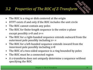
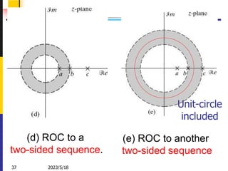
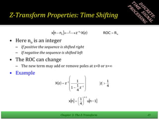
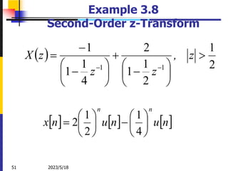
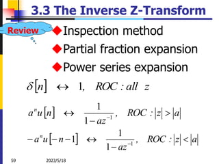
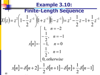
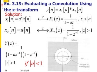
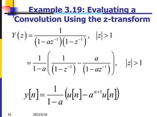
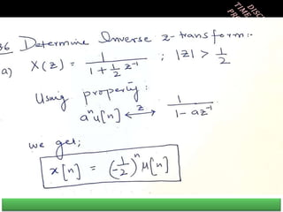
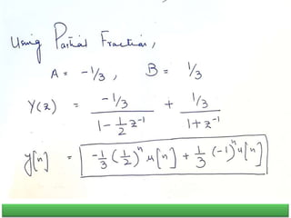
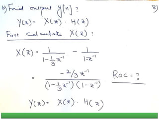
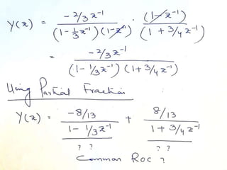
The document summarizes key concepts about the z-transform, which is the discrete-time counterpart of the Laplace transform. It describes the z-transform definition and how it relates to the discrete-time Fourier transform (DTFT). The region of convergence (ROC) is defined as the set of z-values where the z-transform converges. The ROC depends on whether the signal is right-sided, left-sided, or two-sided. Examples are provided to illustrate the ROC for different types of signals. Properties of the ROC like its shape and relationship to system stability and causality are also covered.

1. Chapter 3:
THE Z-TRANSFORM
Content and Figures are from Discrete-Time Signal Processing, 2e by Oppenheim, Shafer and Buck, ©1999-2000 Prentice Hall Inc.

2. 3.1 The Z-Transform
• Counterpart of the Laplace transform for discrete-time signals
• Generalization of the Fourier Transform
Fourier Transform does not converge for all signals
• Definition:
• Compare to DTFT definition:
• z is a complex variable that can be represented as z=r ej
• Substituting z=ej will reduce the z-transform to DTFT
Chapter 3: The Z-Transform 1
   






n
n
z
n
x
z
X
    n
j
n
j
e
n
x
e
X 
 






3.  
   
 
 

j
n
n
z
n
n
re
z
z
n
x
z
X
z
X
n
x
z
X
z
n
x
n
x
















0
)
(
)
(
)
(
3.1 The Z-Transform

4. Z-Transform
   






n
n
z
n
x
z
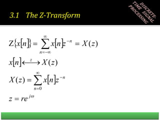
X Bilateral Z-Transform
   
0
n
n
X z x n z



  Unilateral Z-Transform
Clearly, Bilateral and Unilateral Z-Transform are same when x[n] = 0,
for n<0

5.    






n
n
z
n
x
z
X
Z-Transform
    n
j
n
j
e
n
x
e
X 
 






6. • More generally, we can express complex variable
“z” in polar form as:
• With z expressed in this form, Z transform eq. is:
• or
Z-Transform
Again for r=1, this equation reduces to z transform

7. Z-Transform

8. The z-transform and the DTFT
• Convenient to describe on the complex z-plane
• If we plot z=ej for =0 to 2 we get the unit circle
Chapter 3: The Z-Transform 7
Re
Im
Unit Circle

r=1
0
2 0 2
 

j
e
X

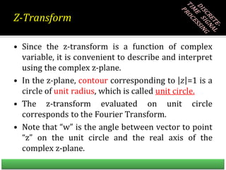
9. Convergence of the z-Transform
• DTFT does not always converge
Example: x[n] = an u[n] for |a|>1 does not have a DTFT
• Complex variable z can be written as r ej so the z-
transform
convert to the DTFT of x[n] multiplied with exponential
sequence r –n
• For certain choices of r the sum
maybe made finite
Chapter 3: The Z-Transform 8
      
 














n
n
j
n
n
n
j
j
e
n
x
e
n
x
re
X 


r
r
    n
j
n
j
e
n
x
e
X 
 





  





n
n
x r n
-

10. Region of Convergence (ROC)
• ROC: The set of values of z for which the z-transform converges
• The region of convergence is made of circles
Chapter 3: The Z-Transform 9
Re
Im
• Example: z-transform converges for
values of 0.5<r<2
ROC is shown on the left
In this example the ROC includes the unit circle,
so DTFT exists

11. Region of Convergence (ROC)

12. Example
 Doesn't converge for any r.
 DTFT exists.
 It has finite energy.
 DTFT converges in a mean square sense.
Example
 Doesn't converge for any r.
 It doesn’t have even finite energy.
 But we define a useful DTFT with impulse
function.
   
n
n
x o

cos

 
sin c n
x n
n



Region of Convergence (ROC)

13. Z Transform of Finite Duration Sequence
   






n
n
z
n
x
z
X

14. Example 1: Right-Sided Exponential Sequence
• For Convergence we require
• Hence the ROC is defined as
• Inside the ROC series converges to
Chapter 3: The Z-Transform 13
         













0
n
n
1
n
n
n
n
az
z
n
u
a
z
X
n
u
a
n
x






0
n
n
1
az
a
z
1
az
n
1




    a
z
z
az
1
1
az
z
X
0
n
1
n
1




 




Re
Im
a 1
o x
• Region outside the circle of
radius “a” is the ROC
• Right-sided sequence, ROCs
extend outside a circle

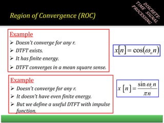
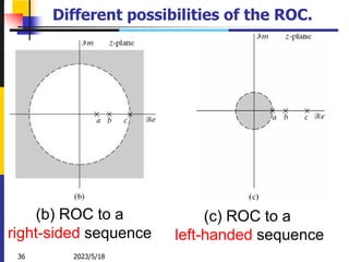
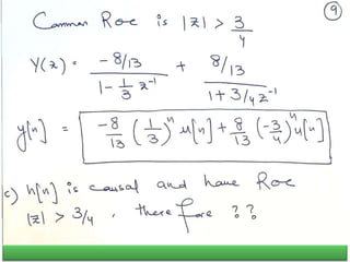
19. Right-Sided Exponential Sequence
If x[n] is a Right Sided Sequence, then ROC will always extend outside the
outermost pole i.e. highest magnitude pole.
In previous example, it has been proven, since the common ROC is Z > 16
Q: Is the system mentioned in Example, a stable system?
A: For a system to be stable, it must include the unit circle. The mentioned
ROC of Z > 16 does not include the unit circle, therefore the system is
unstable.
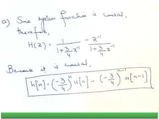
Q: Is the system mentioned in Example, a causal system?
A: For a system to be causal, ROC must extend outside the outermost pole.
The mentioned ROC of Z > 16 shows exactly that, therefore the system is a
causal system

20.    
   
 
a
z
z
az
z
a
z
X
a
z
z
a
z
a
ROC
z
a
z
a
z
a
z
n
u
a
z
X
n
n
n n
n
n
n
n
n
n
n
n












































 


1
1
1
0
1
1 0
1
1
1
1
1
1
1
1
1
:
1
1
   
1



 n
u
a
n
x n
Example 2: Left-Sided Exponential Sequence

21. Example 2: Left-Sided Exponential Sequence
• Region inside the circle of radius “a” is the ROC
• Left-sided sequence, ROCs extend inside the circle

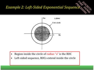
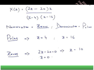
27. Left-Sided Exponential Sequence
If x[n] is a Left Sided Sequence, then ROC will always be inside the innermost
pole i.e. lowest magnitude pole.
In previous example, it has been proven, since the common ROC is Z < 8
Q: Is the system mentioned in Example, a stable system?
A: For a system to be stable, it must include the unit circle. The mentioned
ROC of Z < 8 does include the unit circle, therefore the system is stable.
Q: Is the system mentioned in Example, a causal system?
A: For a system to be causal, ROC must extend outside the outermost pole.
The mentioned ROC of Z < 8 does not show that, therefore the system is non-
causal/ Anti-Causal.

28.      
1
2
1
3
1
















 n
u
n
u
n
x
n
n
 
3
1
3
1
1
1
3
1
1











z
,
z
n
u
Z
n
 
2
1
2
1
1
1
1
2
1
1













z
,
z
n
u
Z
n
 
2
1
3
1
2
1
1
3
1
1
12
1
2
2
1
1
1
3
1
1
1
1
1
1
1
































z
:
ROC
z
z
z
z
z
z
z
X
Solution:
Two Sided Exponential

29. 2023/5/18
28
ROC, pole-zero-plot
     
1
2
1
3
1
















 n
u
n
u
n
x
n
n
 
2
1
3
1
2
1
1
3
1
1
12
1
2
2
1
1
1
3
1
1
1
1
1
1
1
































z
:
ROC
z
z
z
z
z
z
z
X

30. Two-Sided Exponential Sequence

31. 3.2 Properties of The ROC of Z-Transform
• The ROC is a ring or disk centered at the origin
• DTFT exists if and only if the ROC includes the unit circle
• The ROC cannot contain any poles
• The ROC for finite-length sequence is the entire z-plane
except possibly z=0 and z=
• The ROC for a right-handed sequence extends outward from the
outermost pole possibly including z= 
• The ROC for a left-handed sequence extends inward from the
innermost pole possibly including z=0
• The ROC of a two-sided sequence is a ring bounded by poles
• The ROC must be a connected region
• A z-transform does not uniquely determine a sequence without
specifying the ROC
Chapter 3: The Z-Transform 30

32. 2023/5/18
31
Finite-length sequence
     
5


 n
n
n
x 

  0
1 5


 
z
:
ROC
z
z
X
   
2
1
N
n N
n
X z x n z


 
Example :

33. Example 4: Finite Length Sequence
Chapter 3: The Z-Transform 32
 


 



otherwise
0
1
0 N
n
a
n
x
n
N=16
Pole-zero plot
     
 
N
n
u
n
u
a
n
x n



   
0
:
1
1
1
)
(
1
0
1
1
1
1
1
1
0
1
1
0
































z
az
az
ROC
a
z
a
z
z
az
az
az
z
a
z
X
N
n
n
N
N
N
N
N
n
n
N
n
n
n

34. SEQUENCE TRANSFORM ROC
1

z
 
 
0
m
if
or
0
m
if
0
except
z
All



1

z
1
1
1

 z
1
1
1

 z
m
z
 
 
 
 
m
n
n
u
n
u
n






1
1 z
ALL
Some common Z-transform pairs

35.  
 
 
 
 
 
     
 
1
:
cos
2
1
cos
1
cos
:
1
1
:
1
:
1
1
1
:
1
1
2
1
0
1
0
0
2
1
1
2
1
1
1
1




































z
ROC
z
z
z
n
u
n
a
z
ROC
az
az
n
u
na
a
z
ROC
az
az
n
u
na
a
z
ROC
az
n
u
a
a
z
ROC
az
n
u
a
Z
Z
n
Z
n
Z
n
Z
n



Some common Z-transform pairs

36. 2023/5/18
35
Example: Different possibilities of
the ROC define different sequences
A system with three poles

37. 2023/5/18
36
(b) ROC to a
right-sided sequence
Different possibilities of the ROC.
(c) ROC to a
left-handed sequence

38. 2023/5/18
37
(e) ROC to another
two-sided sequence
Unit-circle
included
(d) ROC to a
two-sided sequence.

39. 2023/5/18
38 Zhongguo Liu_Biomedical Engineering_Shandong Univ.
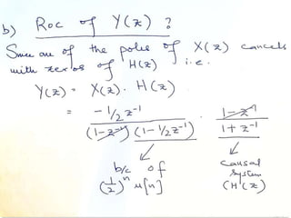
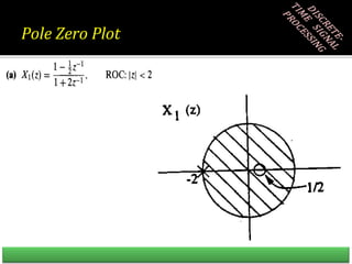
Ex. 3.7 Stability, Causality, and the ROC
Consider a LTI system with impulse
response h[n]. The z-transform of h[n] i.e.
the system function H (z) has the pole-zero
plot shown in Figure. Determine the ROC,
if the system is:
(1) stable system:
(ROC include unit-circle)
(2) causal system:
(right sided sequence)

40. 2023/5/18
39
ROC: , the impulse response is
two-sided, system is non-causal. stable.
Ex. 3.7 Stability, Causality, and the ROC
2
2
1

 z
Solution: (1) stable system (ROC include unit-circle),

41. 2023/5/18
40
ROC: ,the impulse response is right-
sided. system is causal but unstable.
Ex. 3.7 Stability, Causality, and the ROC
2

z
2
1
2
A system is causal
and stable if all the
poles are inside the
unit circle.
(2) causal system: (right sided sequence)

42. 2023/5/18
41
ROC: , the impulse response is
left-sided, system is non-causal, unstable
since the ROC does not include unit circle.
2
1

z
Ex. 3.7 Stability, Causality, and the ROC

43. Stability, Causality, and the ROC
Consider the z-transform X(z) whose pole zero plot is shown in Figure.
i. Determine the ROC of X(z), if it is know that the Fourier transform exists. For
this case, determine whether the system is Right-sided, Left-sided or Two
sided sequence.
ii. How many possible two-sided sequences have the pole zero plot shown in Fig.
iii. Is it possible for a pole zero plot shown in figure to be associated with a system
that is both stable and causal?

44. Stability, Causality, and the ROC

45. 3.4 Z-Transform Properties: Linearity
• Notation
• Linearity
– Note that the ROC of combined sequence may be larger than either ROC
– This would happen if some pole/zero cancellation occurs
– Example:
•Both sequences are right-sided
•Both sequences have a pole z=a
•Both have a ROC defined as |z|>|a|
•In the combined sequence the pole at z=a cancels with a zero at z=a
•The combined ROC is the entire z plane except z=0
Chapter 3: The Z-Transform 44
    x
Z
R
ROC
z
X
n
x 

 

        2
1 x
x
2
1
Z
2
1 R
R
ROC
z
bX
z
aX
n
bx
n
ax 



 


     
N
-
n
u
a
-
n
u
a
n
x n
n


46. Z-Transform Properties: Time Shifting
• Here no is an integer
– If positive the sequence is shifted right
– If negative the sequence is shifted left
• The ROC can change
– The new term may add or remove poles at z=0 or z=
• Example
Chapter 3: The Z-Transform 45
    x
n
Z
o R
ROC
z
X
z
n
n
x o


 

 
 
4
1
z
z
4
1
1
1
z
z
X
1
1

















   
1
-
n
u
4
1
n
x
1
-
n








47. 2023/5/18
46
3.3 The Inverse Z-Transform
Less formal ways are sufficient
and preferable in finding the
inverse z-transform. :
Inspection method
Partial fraction expansion
Power series expansion

48. 2023/5/18
47
3.3 The inverse z-Transform
3.3.1 Inspection Method
  1
1
,
1
Z
n
a u n
az
z a




 
2
1
2
1
1
1
1




z
,
z
z
X
   
n
u
n
x
n







2
1

49. 2023/5/18
48
3.3 The inverse z-Transform
3.3.1 Inspection Method
  1
1
1 ,
1
Z
n
a u n
az
z a

    

 
2
1
2
1
1
1
1




z
,
z
z
X
   
1
2
1









 n
u
n
x
n

50. 2023/5/18
49
3.3 The inverse z-Transform
3.3.2 Partial Fraction Expansion
 
 
 
1
0 0 0 0
1
0
0 0 0
1
1
M
M M
k N M k
k
k k
k k k
N N N
k M N k
k k k
k k k
c z
b z z b z
b
X z
a
a z z a z d z

 
  
  
  

  

  
  
   
1
1
1
1
1
N
k
k k
k k
k
z d
A
d z
w
if M
here A d z X z
N






 



51. 2023/5/18
50 Zhongguo Liu_Biomedical Engineering_Shandong Univ.
Example 3.8
Second-Order z-Transform
 
1 1
1
,
1 1
1 1
2
2
4
1
X z
z z
z
 

  
 
  
 


 

















 1
2
1
1
2
1
1
4
1
1 z
A
z
A
z
X
  1
4
1
1
4
1
1
1 











z
z
X
z
A
  2
2
1
1
2
1
1
2 










z
z
X
z
A

52. 2023/5/18
51
Example 3.8
Second-Order z-Transform
 
2
1
2
1
1
2
4
1
1
1
1
1




















z
,
z
z
z
X
     
n
u
n
u
n
x
n
n














4
1
2
1
2

53. 2023/5/18
52
Example 3.9:
Inverse by Partial Fractions
   
 
1
,
1
2
1
1
1
2
1
2
3
1
2
1
1
1
2
1
2
1
2
1























z
z
z
z
z
z
z
z
z
X

54. 2023/5/18
53
 
1 2
1 2
0 1
1 2 1
1 2
3 1 1 1
1 1
2 2 2
A A
z z
X z B
z
z z z
 

  
 
   

  
2
1
5
2
3
1
2
1
2
3
2
1
1
1
2
1
2
1
2














z
z
z
z
z
z
z
 
 
1
1
1
1
2
1
1
5
1
2















z
z
z
z
X

55. 2023/5/18
54
 
 
1
1 2
1
1
1 1
1 5
2 2
1
1 1
1
1 1
2
2
A A
z
X z
z
z
z z



 
 
    

  
 
 
 
 
9
2
1
1
1
2
1
1
5
1
2
1
1
1
1
1
1 





































z
z
z
z
z
A
 
  8
1
1
2
1
1
5
1
1
1
1
1
1
2 






























z
z
z
z
z
A

56. 2023/5/18
55
 
 
1
1
9 8
2 , 1
1 1
1
2
X z z
z
z


   
  

 
 
 
n
Z

2
2 
  
n
u
z
n
Z














  2
1
2
1
1
1
1
   
n
u
z
Z


 1
1
1
       
n
u
n
u
n
n
x
n
8
2
1
9
2 







 

57. 2023/5/18
56
LTI system Stability, Causality, and ROC
For a LTI system with impulse response h[n],
if it is causal, what do we know about h[n]?
Is h[n] one-sided or two-sided sequence?
Left-sided or right-sided?
 
n
h
 
n
x  
n
y
Then what do we know about the ROC of the
system function H (z)?
If the poles of H (z) are all in the unit circle,
is the system stable?
Review

58. 2023/5/18 Zhongguo Liu_Biomedical Engineering_Shandong Univ.
LTI system Stability, Causality, and ROC
For H (z) with the poles as shown in figure ,
 
   
1 1 1
1
1 1 1
H z
az bz cz
  

  
Unit-circle
included
can we uniquely determine h[n] ?
is the system stable ?
If ROC of H(z) is as shown
in figure, can we uniquely
determine h[n] ?
Review

59. 2023/5/18 Zhongguo Liu_Biomedical Engineering_Shandong Univ.
LTI system Stability, Causality, and ROC
For H (z) with the poles as shown in figure ,
 
   
1 1 1
1
1 1 1
H z
az bz cz
  

  
If the system is causal
(h[n]=0,for n<0,right-sided ),
What’s the ROC like?
If ROC is as shown in
figure, is h[n] one-sided or
two-sided? Is the system
causal or stable?
Review

60. 2023/5/18
59
3.3 The Inverse Z-Transform
Inspection method
Partial fraction expansion
Power series expansion
  z
all
:
ROC
,
n 1


  a
z
:
ROC
,
az
n
u
an





 1
1
1
1
  a
z
:
ROC
,
az
n
u
an


 1
1
1
Review

61. 2023/5/18
60
Example 3.10:
Finite-Length Sequence
     1
2
1
1
1
2
2
1
1
2
1
1
1
2
1
1 
















 z
z
z
z
z
z
z
z
X
 


















otherwise
n
n
n
n
n
x
,
0
1
,
2
1
0
,
1
1
,
2
1
2
,
1
         
1
2
1
1
2
1
2 





 n
n
n
n
n
x 




62. 2023/5/18
61
Ex. 3.19: Evaluating a Convolution Using
the z-transform
   
1
n
x n a u n

   
2
x n u n

1
if a 
 
Y z 
  
1 1
1
1 1
1
az z
z
 
 

     
1 2
*
y n x n x n

 
1 1
1
,
1
Z
X z z a
az

  

 
2 1
1
, 1
1
Z
X z z
z

  

Solution:

63. 2023/5/18
62
Example 3.19: Evaluating a
Convolution Using the z-transform
 
  
   
1 1
1 1
1
, 1
1 1
1 1
, 1
1 1 1
Y z z
az z
a
z
a z az
 
 
 
 
 
 
  
 
  
 
     
 
n
u
a
n
u
a
n
y n 1
1
1 




64. 2023/5/18
63

81. Pole Zero Plot
Determine Pole Zero Plots of Following Sequences

82. Pole Zero Plot

83. Pole Zero Plot

84. Pole Zero Plot
• Poles: 2/3 and 3/2
• Zeros: 1 and -2