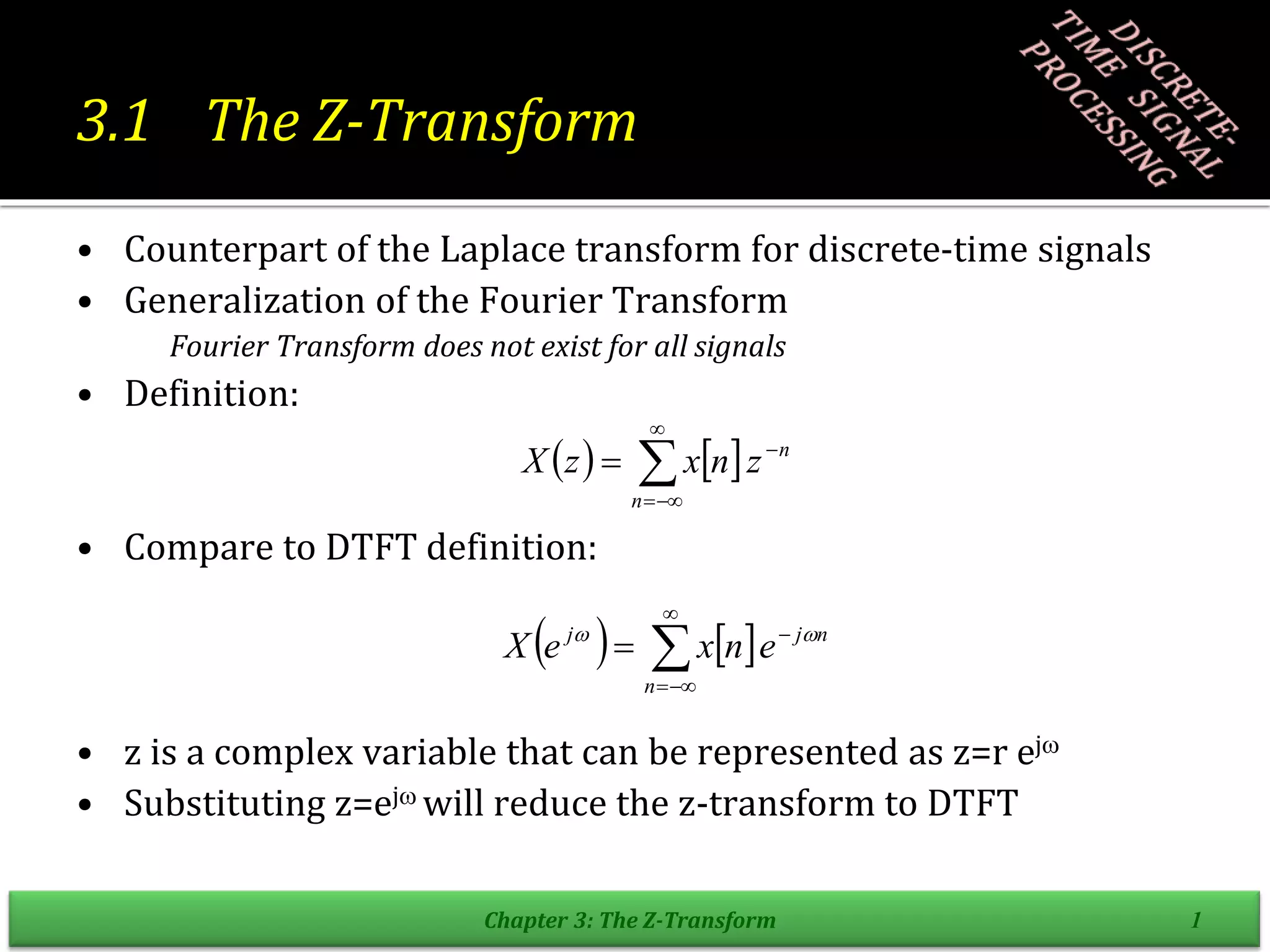
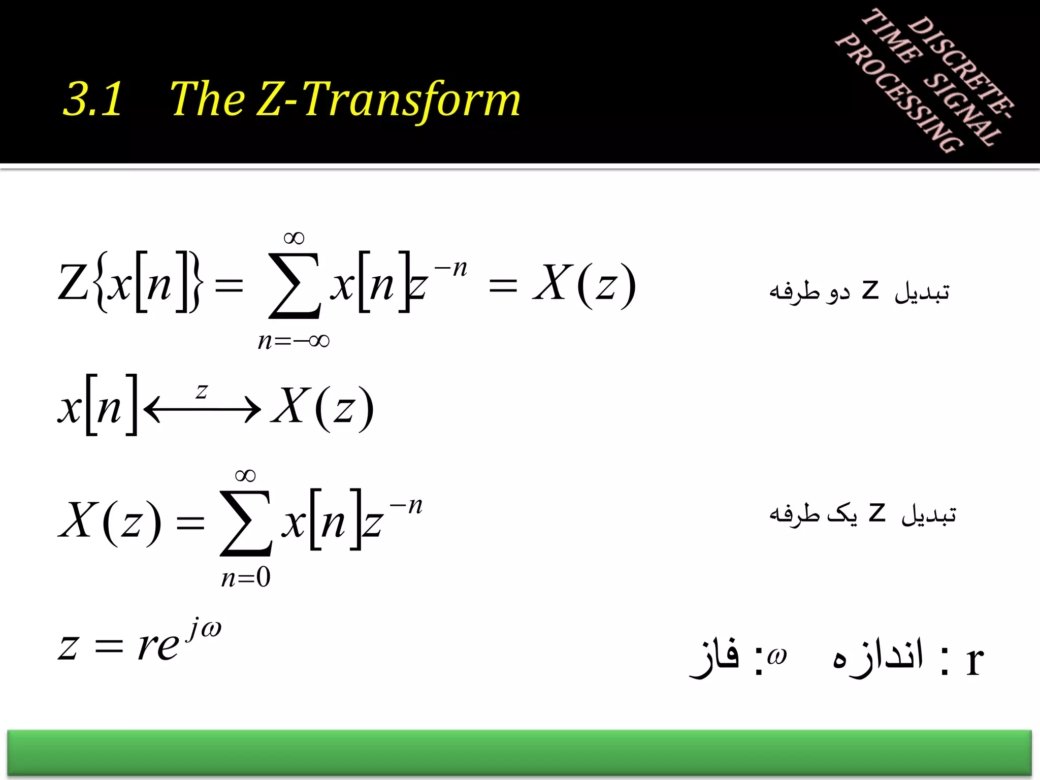
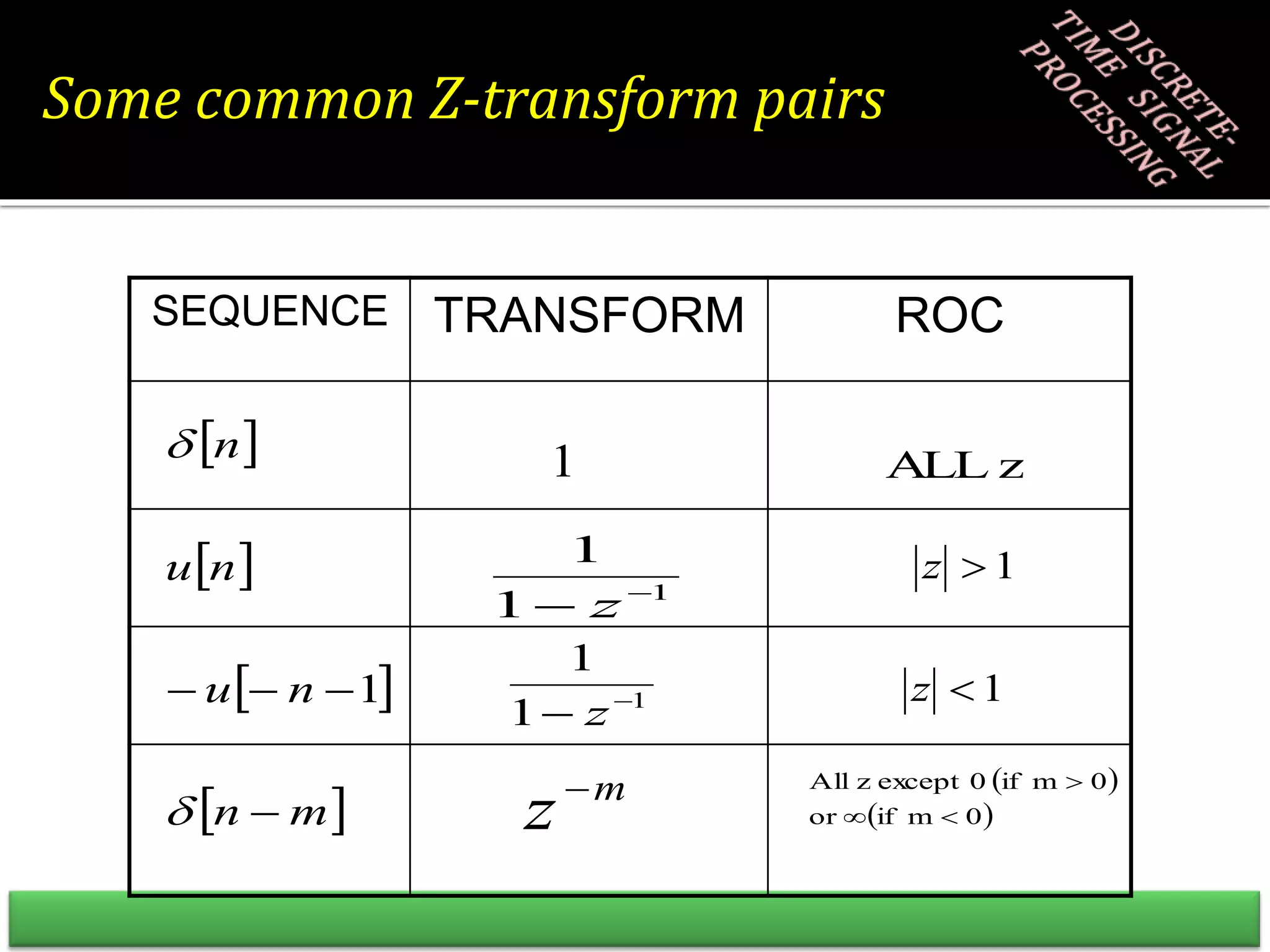
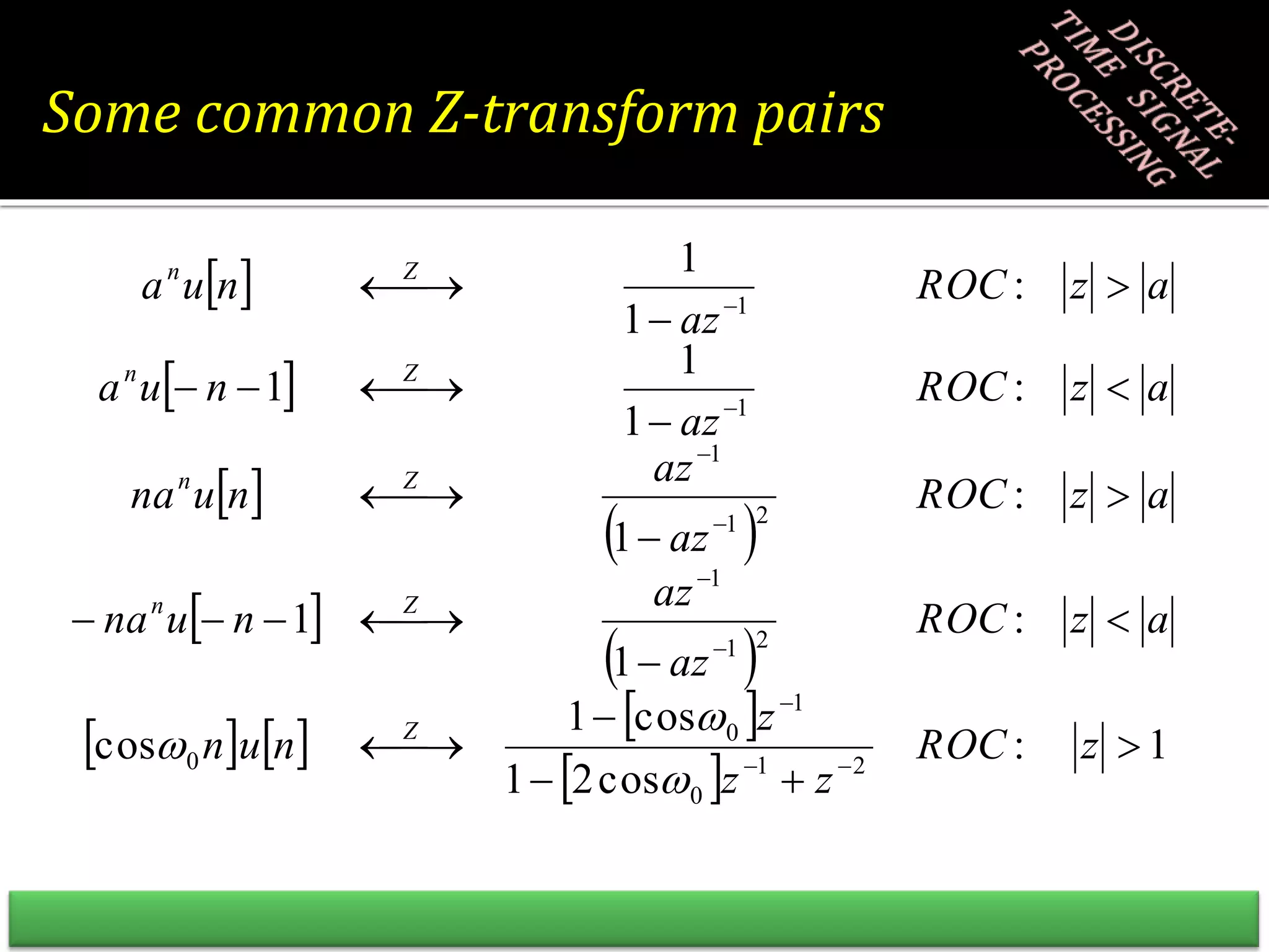
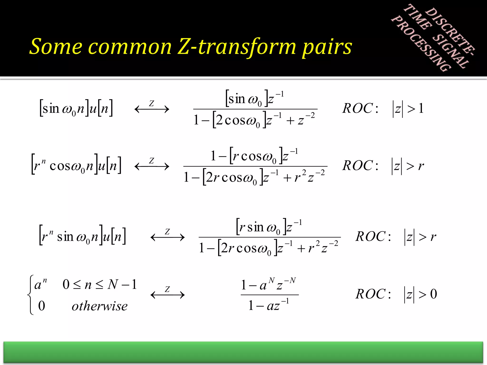
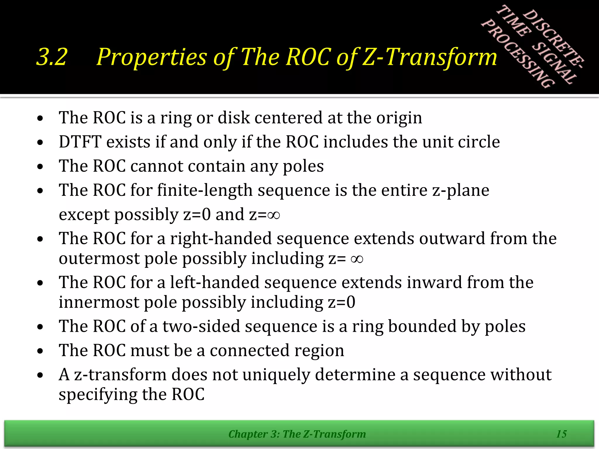
The document summarizes key concepts about the z-transform, which is the discrete-time counterpart of the Laplace transform. It defines the z-transform, compares it to the discrete-time Fourier transform (DTFT), and discusses its region of convergence (ROC). Examples are provided to illustrate ROCs for different types of sequences, including right-sided, left-sided, and two-sided exponential sequences as well as a finite-length sequence. Common z-transform pairs are also listed.

1. Department of Computer Eng.
Sharif University of Technology
Discrete-time signal processing
Chapter 3:
THE Z-TRANSFORM
Content and Figures are from Discrete-Time Signal Processing, 2e by Oppenheim, Shafer and Buck, ©1999-2000 Prentice Hall Inc.

2. 3.1 The Z-Transform
• Counterpart of the Laplace transform for discrete-time signals
• Generalization of the Fourier Transform
Fourier Transform does not exist for all signals
• Definition:
• Compare to DTFT definition:
• z is a complex variable that can be represented as z=r ej
• Substituting z=ej will reduce the z-transform to DTFT
Chapter 3: The Z-Transform 1
   






n
n
z
n
x
z
X
    n
j
n
j
e
n
x
e
X 
 






3.  
   
 
 

j
n
n
z
n
n
re
z
z
n
x
z
X
z
X
n
x
z
X
z
n
x
n
x
















0
)
(
)
(
)
(
r
:
‫اندازه‬
:
‫فاز‬ 
‫تبدیل‬
z
‫طرفه‬‫یک‬
‫تبدیل‬
z
‫طرفه‬‫دو‬
3.1 The Z-Transform

4. The z-transform and the DTFT
• Convenient to describe on the complex z-plane
• If we plot z=ej for =0 to 2 we get the unit circle
Chapter 3: The Z-Transform 3
Re
Im
Unit Circle

r=1
0
2 0 2
 

j
e
X

5. Convergence of the z-Transform
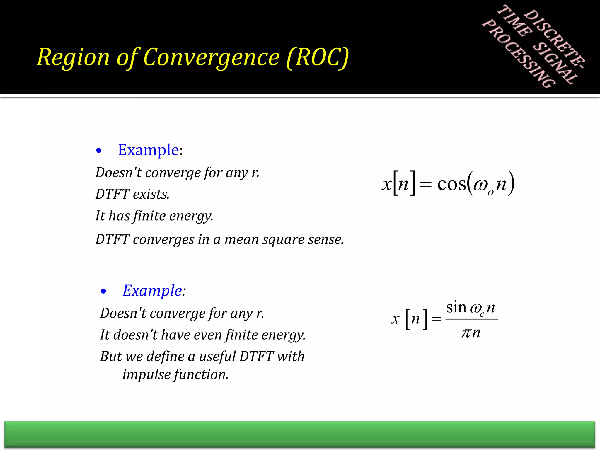
• DTFT does not always converge
Example: x[n] = anu[n] for |a|>1 does not have a DTFT
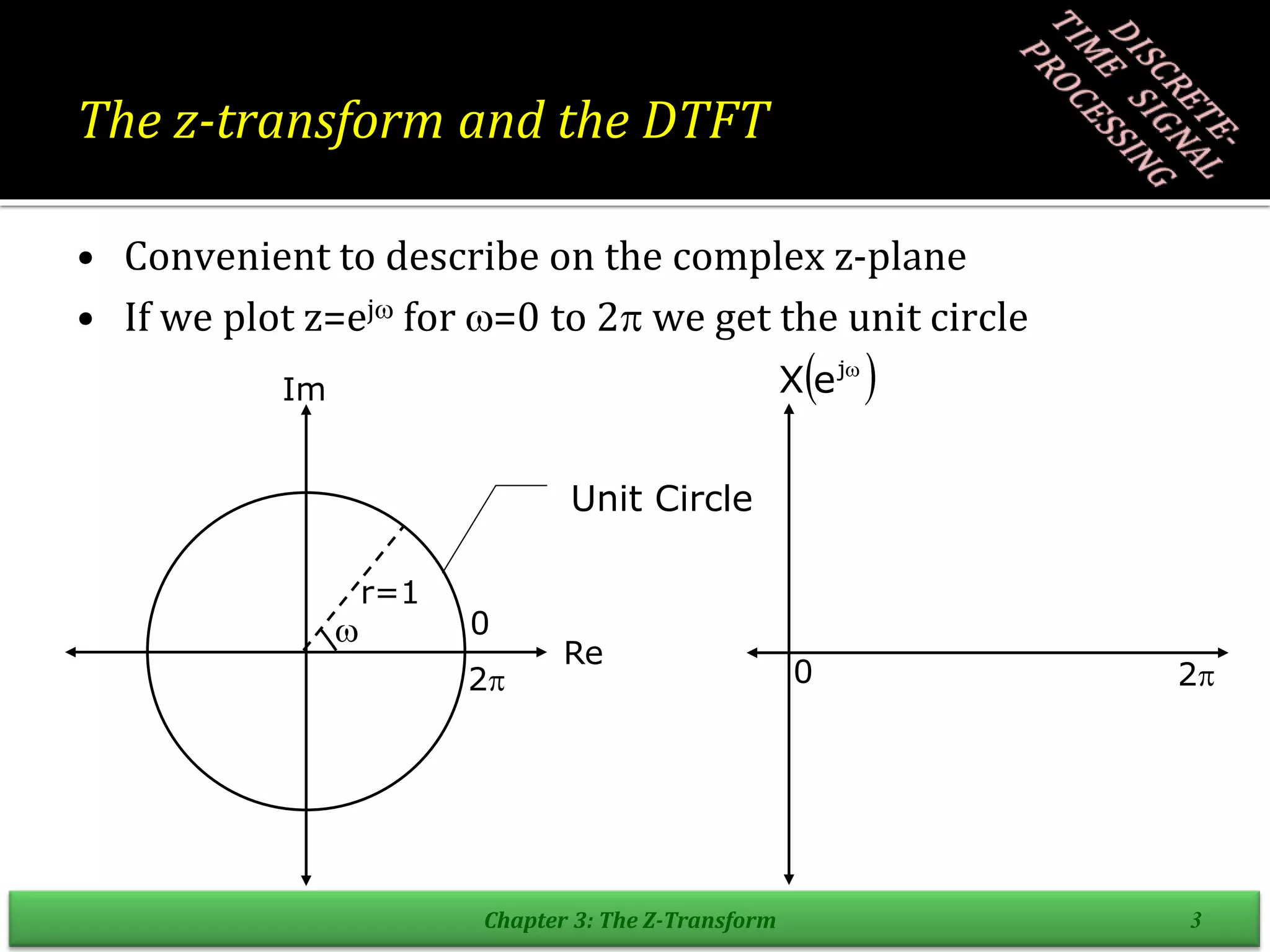
• Complex variable z can be written as r ej so the z-
transform
convert to the DTFT of x[n] multiplied with exponential
sequence r –n
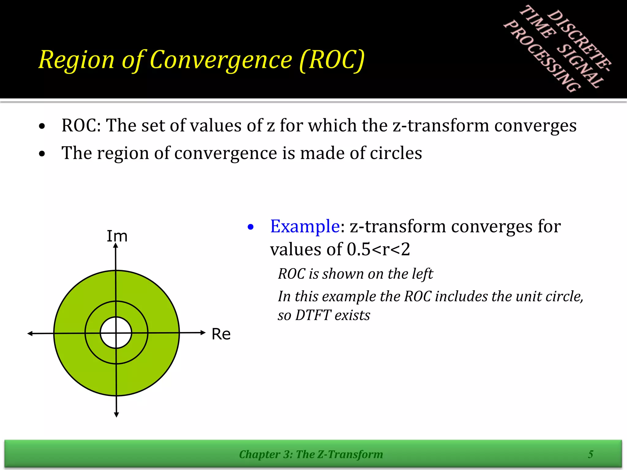
• For certain choices of r the sum
maybe made finite
Chapter 3: The Z-Transform 4
      
 














n
n
j
n
n
n
j
j
e
n
x
e
n
x
re
X 


r
r
    n
j
n
j
e
n
x
e
X 
 





  





n
n
x r n
-

6. Region of Convergence (ROC)
• ROC: The set of values of z for which the z-transform converges
• The region of convergence is made of circles
Chapter 3: The Z-Transform 5
Re
Im
• Example: z-transform converges for
values of 0.5<r<2
ROC is shown on the left
In this example the ROC includes the unit circle,
so DTFT exists

7. • Example:
Doesn't converge for any r.
DTFT exists.
It has finite energy.
DTFT converges in a mean square sense.
• Example:
Doesn't converge for any r.
It doesn’t have even finite energy.
But we define a useful DTFT with
impulse function.
   
n
n
x o

cos

 
sin c n
x n
n



Region of Convergence (ROC)

8. Example 1: Right-Sided Exponential Sequence
• For Convergence we require
• Hence the ROC is defined as
• Inside the ROC series converges to
Chapter 3: The Z-Transform 7
         













0
n
n
1
n
n
n
n
az
z
n
u
a
z
X
n
u
a
n
x






0
n
n
1
az
a
z
1
az
n
1




    a
z
z
az
1
1
az
z
X
0
n
1
n
1




 




Re
Im
a 1
o x
• Region outside the circle of
radius a is the ROC
• Right-sided sequence ROCs
extend outside a circle

9. (
‫ا‬‫ر‬‫چپگ‬‫دنباله‬
)
   
   
 
a
z
z
az
z
a
z
X
a
z
z
a
z
a
ROC
z
a
z
a
z
a
z
n
u
a
z
X
n
n
n n
n
n
n
n
n
n
n
n












































 


1
1
1
0
1
1 0
1
1
1
1
1
1
1
1
1
:
1
1
   
1



 n
u
a
n
x n
Example 2: Left-Sided Exponential Sequence

10. Example 3: Two-Sided Exponential Sequence
Chapter 3: The Z-Transform 9
     
1
-
n
-
u
2
1
-
n
u
3
1
n
x
n
n














1
1
1
0
1
0
1
3
1
1
1
3
1
1
3
1
3
1
3
1



































z
z
z
z
z
n
n
1
1
0
1
1
1
n
n
1
z
2
1
1
1
z
2
1
1
z
2
1
z
2
1
z
2
1


































z
3
1
1
z
3
1
:
ROC 1


 
z
2
1
1
z
2
1
:
ROC 1



 




























2
1
z
3
1
z
12
1
z
z
2
z
2
1
1
1
z
3
1
1
1
z
X
1
1
Im
2
1
oo
12
1
x
x
3
1


11. Example 4: Finite Length Sequence
Chapter 3: The Z-Transform 10
 


 



otherwise
0
1
0 N
n
a
n
x
n
N=16
Pole-zero plot
     
 
N
n
u
n
u
a
n
x n



   
0
:
1
1
1
)
(
1
0
1
1
1
1
1
1
0
1
1
0
































z
az
az
ROC
a
z
a
z
z
az
az
az
z
a
z
X
N
n
n
N
N
N
N
N
n
n
N
n
n
n

12. Some common Z-transform pairs
Chapter 3: The Z-Transform 11

13. SEQUENCE TRANSFORM ROC
1

z
 
 
0
m
if
or
0
m
if
0
except
z
All



1

z
1
1
1

 z
1
1
1

 z
m
z
 
 
 
 
m
n
n
u
n
u
n






1
1 z
ALL
Some common Z-transform pairs

14.  
 
 
 
 
 
     
 
1
:
cos
2
1
cos
1
cos
:
1
1
:
1
:
1
1
1
:
1
1
2
1
0
1
0
0
2
1
1
2
1
1
1
1




































z
ROC
z
z
z
n
u
n
a
z
ROC
az
az
n
u
na
a
z
ROC
az
az
n
u
na
a
z
ROC
az
n
u
a
a
z
ROC
az
n
u
a
Z
Z
n
Z
n
Z
n
Z
n



Some common Z-transform pairs

15.      
 
0
:
1
1
0
1
0
:
cos
2
1
sin
sin
1
2
2
1
0
1
0
0







 












z
ROC
az
z
a
otherwise
N
n
a
r
z
ROC
z
r
z
r
z
r
n
u
n
r
N
N
Z
n
Z
n



     
 
     
 
r
z
ROC
z
r
z
r
z
r
n
u
n
r
z
ROC
z
z
z
n
u
n
Z
n
Z

















:
cos
2
1
cos
1
cos
1
:
cos
2
1
sin
sin
2
2
1
0
1
0
0
2
1
0
1
0
0






Some common Z-transform pairs

16. 3.2 Properties of The ROC of Z-Transform
• The ROC is a ring or disk centered at the origin
• DTFT exists if and only if the ROC includes the unit circle
• The ROC cannot contain any poles
• The ROC for finite-length sequence is the entire z-plane
except possibly z=0 and z=
• The ROC for a right-handed sequence extends outward from the
outermost pole possibly including z= 
• The ROC for a left-handed sequence extends inward from the
innermost pole possibly including z=0
• The ROC of a two-sided sequence is a ring bounded by poles
• The ROC must be a connected region
• A z-transform does not uniquely determine a sequence without
specifying the ROC
Chapter 3: The Z-Transform 15

17. Stability, Causality, and the ROC
• Consider a system with impulse response h[n]
• The z-transform H(z) and the pole-zero plot shown below
• Without any other information h[n] is not uniquely determined
|z|>2 or |z|<½ or ½<|z|<2
• If system stable ROC must include unit-circle: ½<|z|<2
• If system is causal must be right sided: |z|>2
Chapter 3: The Z-Transform 16

18. 3.4 Z-Transform Properties: Linearity
• Notation
• Linearity
– Note that the ROC of combined sequence may be larger than either ROC
– This would happen if some pole/zero cancellation occurs
– Example:
•Both sequences are right-sided
•Both sequences have a pole z=a
•Both have a ROC defined as |z|>|a|
•In the combined sequence the pole at z=a cancels with a zero at z=a
•The combined ROC is the entire z plane except z=0
Chapter 3: The Z-Transform 17
    x
Z
R
ROC
z
X
n
x 

 

        2
1 x
x
2
1
Z
2
1 R
R
ROC
z
bX
z
aX
n
bx
n
ax 



 


     
N
-
n
u
a
-
n
u
a
n
x n
n


19. Z-Transform Properties: Time Shifting
• Here no is an integer
– If positive the sequence is shifted right
– If negative the sequence is shifted left
• The ROC can change
– The new term may add or remove poles at z=0 or z=
• Example
Chapter 3: The Z-Transform 18
    x
n
Z
o R
ROC
z
X
z
n
n
x o


 

 
 
4
1
z
z
4
1
1
1
z
z
X
1
1

















   
1
-
n
u
4
1
n
x
1
-
n








20. Z-Transform Properties: Multiplication by
Exponential
• ROC is scaled by |zo|
• All pole/zero locations are scaled
• If zo is a positive real number: z-plane shrinks or expands
• If zo is a complex number with unit magnitude it rotates
• Example: We know the z-transform pair
• Let’s find the z-transform of
Chapter 3: The Z-Transform 19
    x
o
o
Z
n
o R
z
ROC
z
/
z
X
n
x
z 

 

  1
z
:
ROC
z
-
1
1
n
u 1
-
Z


 

             
n
u
re
2
1
n
u
re
2
1
n
u
n
cos
r
n
x
n
j
n
j
o
n o
o 






  r
z
z
re
1
2
/
1
z
re
1
2
/
1
z
X 1
j
1
j o
o




 





21. Z-Transform Properties: Differentiation
• Example: We want the inverse z-transform of
• Let’s differentiate to obtain rational expression
• Making use of z-transform properties and ROC
Chapter 3: The Z-Transform 20
   
x
Z
R
ROC
dz
z
dX
z
n
nx 


 

    a
z
az
1
log
z
X 1


 
   
1
1
1
2
az
1
1
az
dz
z
dX
z
az
1
az
dz
z
dX











     
1
n
u
a
a
n
nx
1
n




     
1
n
u
n
a
1
n
x
n
1
n





22. Z-Transform Properties: Conjugation
Chapter 3: The Z-Transform 21
    x
*
*
Z
*
R
ROC
z
X
n
x 

 

   
     
         
 
n
n
n n
n n
n n
n n
X z x n z
X z x n z x n z
X z x n z x n z Z x n




 
  
 
 

     
 

 
 
 
 
  

 
 

23. Z-Transform Properties: Time Reversal
• ROC is inverted
• Example:
• Time reversed version of
Chapter 3: The Z-Transform 22
   
x
Z
R
1
ROC
z
/
1
X
n
x 

 


   
n
u
a
n
x n

 
 
n
u
an
  1
1
1
-
1
-1
a
z
z
a
-
1
z
a
-
az
1
1
z
X 







24. Z-Transform Properties: Convolution
• Convolution in time domain is multiplication in z-domain
• Example: Let’s calculate the convolution of
• Multiplications of z-transforms is
• ROC: if |a|<1 ROC is |z|>1 if |a|>1 ROC is |z|>|a|
• Partial fractional expansion of Y(z)
Chapter 3: The Z-Transform 23
        2
x
1
x
2
1
Z
2
1 R
R
:
ROC
z
X
z
X
n
x
n
x 

 


       
n
u
n
x
and
n
u
a
n
x 2
n
1 

  a
z
:
ROC
az
1
1
z
X 1
1 

 
  1
z
:
ROC
z
1
1
z
X 1
2 

 
     
  
1
1
2
1
z
1
az
1
1
z
X
z
X
z
Y 





  1
z
:
ROC
assume
1
1
1
1
1
1
1











 

az
a
z
a
z
Y      
 
n
u
a
n
u
a
1
1
n
y 1
n




25. Some Z-transform properties
Chapter 3: The Z-Transform 24

26. 3.3 The Inverse Z-Transform
• Formal inverse z-transform is based on a Cauchy integral
• Less formal ways sufficient most of the time
– Inspection method
– Partial fraction expansion
– Power series expansion
• Inspection Method
Make use of known z-transform pairs such as
Example: The inverse z-transform of
Chapter 3: The Z-Transform 25
  a
z
az
1
1
n
u
a 1
Z
n



 
 
     
n
u
2
1
n
x
2
1
z
z
2
1
1
1
z
X
n
1













27. Inverse Z-Transform by Partial Fraction
Expansion
• Assume that a given z-transform can be expressed as
• Apply partial fractional expansion
• First term exist only if M>N
– Br is obtained by long division
• Second term represents all first order poles
• Third term represents an order s pole
– There will be a similar term for every high-order pole
• Each term can be inverse transformed by inspection
Chapter 3: The Z-Transform 26
 






 N
0
k
k
k
M
0
k
k
k
z
a
z
b
z
X
 
 


 












s
1
m
m
1
i
m
N
i
k
,
1
k
1
k
k
N
M
0
r
r
r
z
d
1
C
z
d
1
A
z
B
z
X

28. Inverse Z-Transform by Partial Fraction
Expansion
• Coefficients are given as
• Easier to understand with examples
Chapter 3: The Z-Transform 27
 
 


 












s
1
m
m
1
i
m
N
i
k
,
1
k
1
k
k
N
M
0
r
r
r
z
d
1
C
z
d
1
A
z
B
z
X
    k
d
z
1
k
k z
X
z
d
1
A 



   
   
  1
i
d
w
1
s
i
m
s
m
s
m
s
i
m w
X
w
d
1
dw
d
d
!
m
s
1
C

















29. Example 5: 2nd Order Z-Transform
Chapter 3: The Z-Transform 28
 
2
1
z
:
ROC
z
2
1
1
z
4
1
1
1
z
X
1
1


















 

















 1
2
1
1
z
2
1
1
A
z
4
1
1
A
z
X
  1
4
1
2
1
1
1
z
X
z
4
1
1
A 1
4
1
z
1
1 
























 


  2
2
1
4
1
1
1
z
X
z
2
1
1
A 1
2
1
z
1
2 























 



30. Example 5 Continued
• ROC extends to infinity
– Indicates right sided sequence
Chapter 3: The Z-Transform 29
 
2
1
z
z
2
1
1
2
z
4
1
1
1
z
X
1
1




















     
n
u
4
1
-
n
u
2
1
2
n
x
n
n














31. Example 6
• Long division to obtain Bo
Chapter 3: The Z-Transform 30
   
 
1
z
z
1
z
2
1
1
z
1
z
2
1
z
2
3
1
z
z
2
1
z
X
1
1
2
1
2
1
2
1























1
z
5
2
z
3
z
2
1
z
2
z
1
z
2
3
z
2
1
1
1
2
1
2
1
2














 
 
1
1
1
z
1
z
2
1
1
z
5
1
2
z
X















  1
2
1
1
z
1
A
z
2
1
1
A
2
z
X 
 




  9
z
X
z
2
1
1
A
2
1
z
1
1 











    8
z
X
z
1
A
1
z
1
2 





32. Example 5 Continued
• ROC extends to infinity
– Indicates right-sided sequence
Chapter 3: The Z-Transform 31
  1
z
z
1
8
z
2
1
1
9
2
z
X 1
1





 

       
n
8u
-
n
u
2
1
9
n
2
n
x
n










33. Inverse Z-Transform by Power Series
Expansion
• The z-transform is power series
• In expanded form
• Z-transforms of this form can generally be inversed easily
• Especially useful for finite-length series
Chapter 3: The Z-Transform 32
   






n
n
z
n
x
z
X
            
 







 
 2
1
1
2
2
1
0
1
2 z
x
z
x
x
z
x
z
x
z
X

34.     
1
2
1
1
1
2
z
2
1
1
z
2
1
z
z
1
z
1
z
2
1
1
z
z
X


















         
1
n
2
1
n
1
n
2
1
2
n
n
x 










 



















2
n
0
1
n
2
1
0
n
1
1
n
2
1
2
n
1
n
x
Example 6