Download to read offline
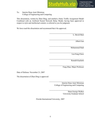


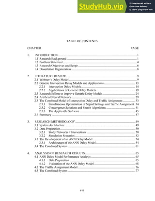

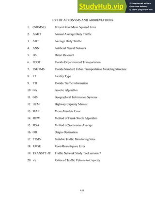

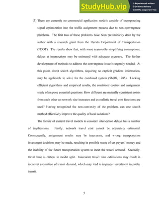
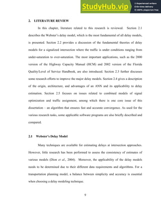


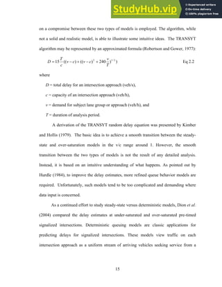

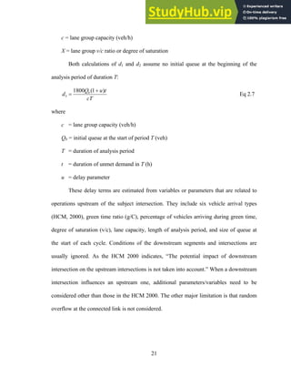
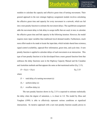
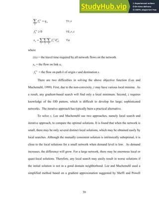
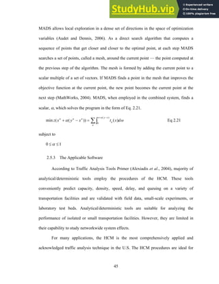
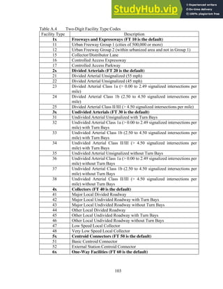
![d = control delay per vehicle (s/veh)
d1 = uniform control delay assuming uniform arrivals (s/veh)
PF = uniform delay progression adjustment factor accounting for effects of signal
progression
d2 = incremental delay to account for effect of random arrivals and over-saturation
queues
d3 = initial queue delay accounting for delay to all vehicles in analysis period due to
initial queue at start of analysis period (s/veh)
In Eq. 2.4, d1 and d2 are defined as follows:
⎟
⎠
⎞
⎜
⎝
⎛
×
−
−
×
=
C
g
X
C
g
C
d
)
,
1
min(
1
2
)
1
( 2
1 Eq 2.5
where
C = cycle length(s)
g = effective green time
X = v/c ratio or degree of saturation for lane group
and
d2 = 900T [(X – 1) +
cT
X
kl
)
(X 8
1 2
+
− ] Eq. 2.6
where
T = duration of analysis period
k = incremental delay factor dependent on controller settings
l = upstream filtering/metering adjustment factor
20](https://image.slidesharecdn.com/astatictrafficassignmentmodelcombinedwithanartificialneuralnetworkdelaymodel-230806163824-28972993/85/A-Static-Traffic-Assignment-Model-Combined-With-An-Artificial-Neural-Network-Delay-Model-34-320.jpg)
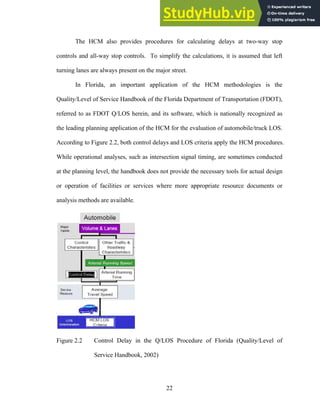

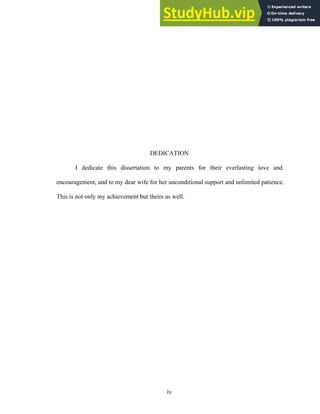
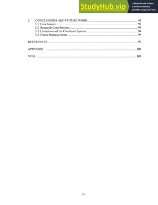
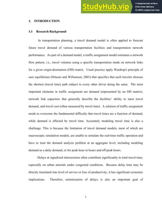
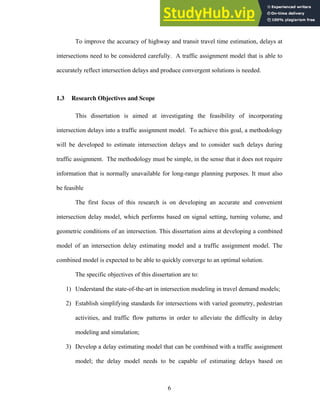
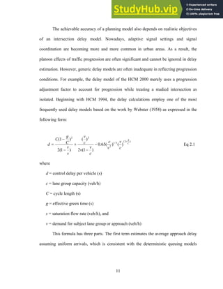
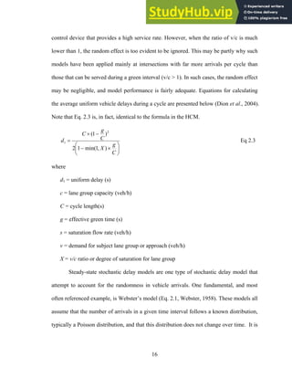
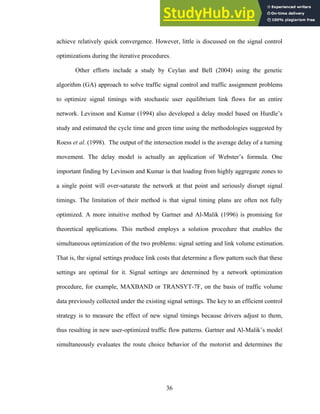
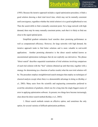
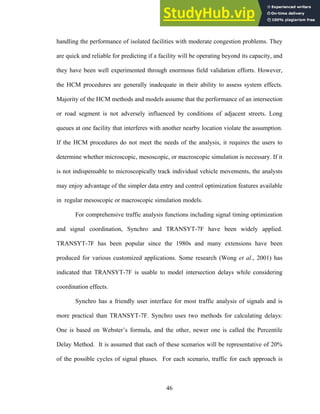
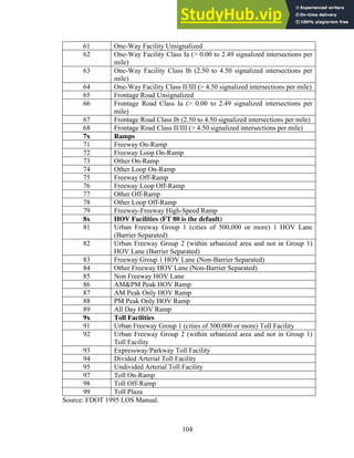
![is an initial queue, the HCM 2000 delay model yields the same uniform delay values for
all arrival types, which does not seem reasonable because platooning affects delay.
Benekohal and Kim propose a new uniform delay model considering platoon impact for
over-saturated traffic conditions when progression is poor. This approach directly
quantifies the platooning effects in delay, eliminating the need to apply a progression
adjustment factor. Like the HCM 2000, the proposed model is applicable with or without
an initial queue:
d1 = 0.5sg [Q1C + Q2(C-t1) – qoC2
– sg2
] Eq 2.8
where
qav = average arrival rate (veh/s)
qpl = platoon arrival rate (veh/s)
qn = non-platoon arrival rate (veh/s)
t1 = platoon duration time (s)
qo = overflow rate (qav minus c) (veh/s)
Q1 = number of arrivals when queue increase rate changes for the first time (= qp t1)
Q2 = number of arrivals at the end of cycle (= qavC)
Compared to inputs in the HCM, this arrival based model also requires platoon
duration time (t1), platoon flow rate (qpl), and non-platoon flow rate (qn) for calculating
platoon and non-platoon arrival rates and compute the delay. The additional input may be
difficult to collect from the planning perspective. However, the authors declared that this
arrival-based approach was more accurate than the HCM approach.
Another major limitation of the HCM methodologies is that its delay model only
deals with isolated intersections. At present, most delay models deal with congestion
25](https://image.slidesharecdn.com/astatictrafficassignmentmodelcombinedwithanartificialneuralnetworkdelaymodel-230806163824-28972993/85/A-Static-Traffic-Assignment-Model-Combined-With-An-Artificial-Neural-Network-Delay-Model-39-320.jpg)
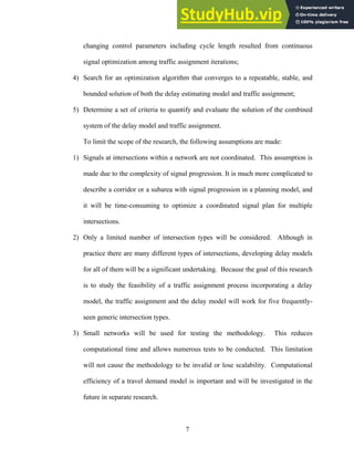
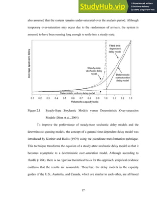
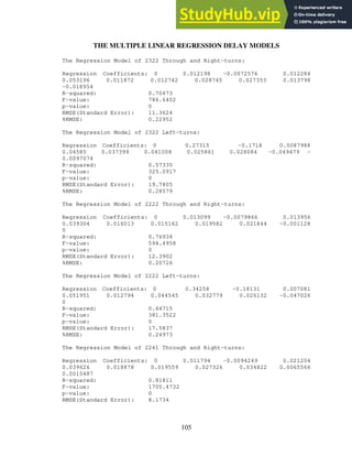
![)]
1
1
(
)
1
(
2
[
2 1
1
)
4
(
4 1
λ
−
−
+
=
v
h
n
d
n
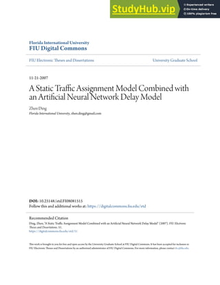
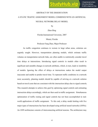
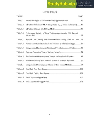
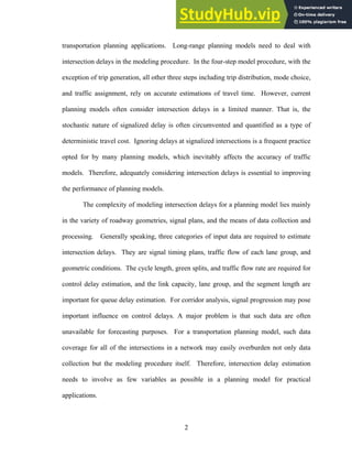
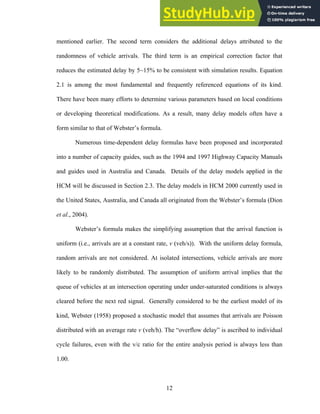
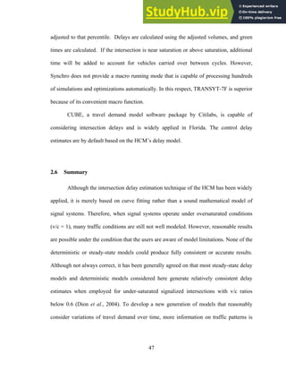
d v Eq 2.9
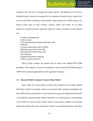
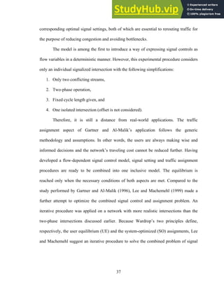
where
n = total number of vehicles queued at the upstream intersection
hv = effective space headway (m)
1
v = speed of mid-block stopping wave (m/s)
1
λ = speed of mid-block starting wave (m/s)
1
)
4
(
d = portion of d4 incurred by the first vehicle at an upstream intersection
)
(
1
2
2
1
2
2
1
)
4
( 1
λ
L
v
L
off
v
L
v
L
d
a
−
−
+
+
= Eq 2.10
where
Off = offset (s)
L1 = queue length measured from the downstream intersection stop line to the tail of
the queue (m)
L2 = remaining space on link (not occupied by vehicles) (m)
v1 = speed of mid-block starting wave (m/s)
v2 = speed of starting wave at downstream intersection (m/s).
va = average link speed (m/s)
Because the queue length at the downstream approach directly impacts the
magnitude of d4, the model needs to include parameters such as offsets, incoming volume
from the upstream intersection, and other traffic control variables. Due to the many
variables involved, including green/red phase, offsets, and average link speed, data
requirements at this level of detail may overburden the transportation planning model.
27](https://image.slidesharecdn.com/astatictrafficassignmentmodelcombinedwithanartificialneuralnetworkdelaymodel-230806163824-28972993/85/A-Static-Traffic-Assignment-Model-Combined-With-An-Artificial-Neural-Network-Delay-Model-41-320.jpg)

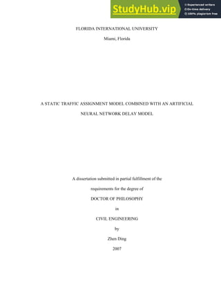
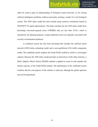
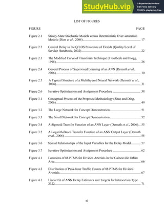
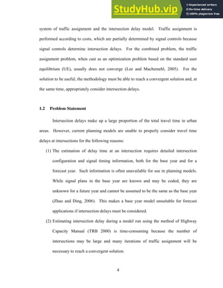
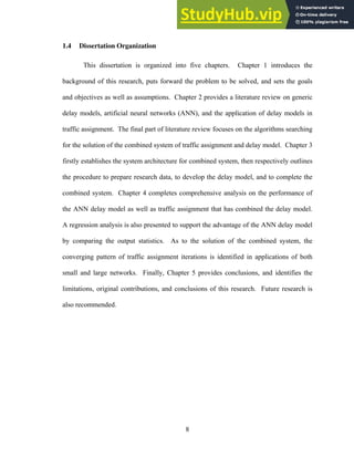
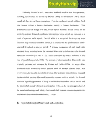
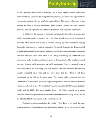
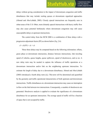
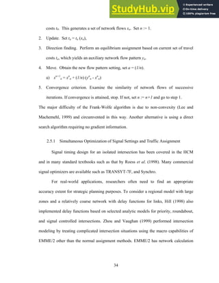
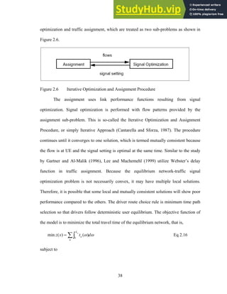
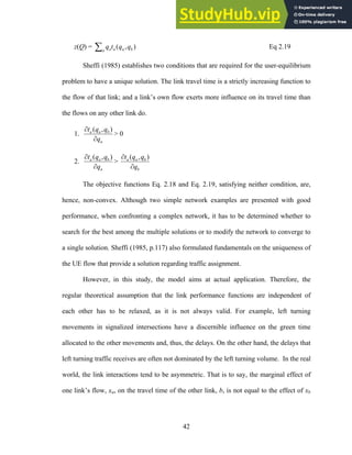
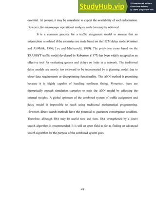
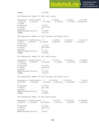
![j=1
where
Ni = net input signal (level of internal activity) in node i,
Wij = connection weight between artificial neurons i and j,
Xj = value of signal coming from previous node j,
bi = bias term of node i (corresponds to an activation threshold),
n = number of input signals from previous nodes.
When the weighted sum of the input signals exceeds the activation threshold bi,
the artificial neuron outputs a signal yi dictated by a transfer function f(x). The output
signal is then expressed as a function of the input signal Ni by:
yi = f (Ni) Eq 2.14
where
f(x) = 1 / (1 + e-x
), may be a sigmoid function which accepts input over the range (-
∞, +∞) and uniquely maps the output yi into the range [0,1].
The neural network modifies the connection weights between the layers and the
node biases in ensuing iterations to allow a type of learning for the network. The weights
and node biases are shifted until the error between the desired output and the actual
output is minimized. Learning (or training) is the process whose objective is to adjust the
link weights and node biases so that when presented with a set of inputs, ANN produces
the desired outputs.
In recent years, artificial neural networks (ANNs) have been frequently employed
in classification, optimization, and prediction. ANNs are suitable in such circumstances
to predict the behavior where cause and effect relationships are little known. ANNs also
32](https://image.slidesharecdn.com/astatictrafficassignmentmodelcombinedwithanartificialneuralnetworkdelaymodel-230806163824-28972993/85/A-Static-Traffic-Assignment-Model-Combined-With-An-Artificial-Neural-Network-Delay-Model-46-320.jpg)

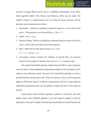
![2. For a large number of direct search methods, it is possible to provide rigorous
guarantees of convergence.
A preliminary study has been performed using the direct search method to find at
least a local optimum. The local optimum ensures the equilibrium between traffic
assignment and signal controls. In other words, the signal timings optimized are not
affected by the negligible change of the assigned volume, and so it is with intersection
delays. The issues regarding the applied optimization search algorithm in the model will
provide solid proof of convergence and the relevance to real-world applications.
2.5.2 Convergence Solutions and Search Algorithms
The combined system aims at solving Eq. 2.16. The calculation is developed from
a link travel cost calculation. The link flow on a single link may be calculated as
∑∑∑
=
m n k
mn
ak
mn
k
a P
q δ Eq 2.17
where
mn
ak
δ = 1 if link a is on path k and 0 otherwise
mn
k
P = flow on route k connecting OD pair (m, n)
mn
f = trip demand rate between origin m and destination n
If denotes the average travel time on link a (q
)
,
( b
a
a q
q
t b denotes the conflicting
flow on link b), the user equilibrium objective function is
z(Q) = ∑ ∫
∫ +
a
q
a
q
b
a
a
a
dw
w
t
dw
q
w
t
0
0
)
0
,
(
)
,
(
[
2
1
] Eq 2.18
and the corresponding system optimization function is
41](https://image.slidesharecdn.com/astatictrafficassignmentmodelcombinedwithanartificialneuralnetworkdelaymodel-230806163824-28972993/85/A-Static-Traffic-Assignment-Model-Combined-With-An-Artificial-Neural-Network-Delay-Model-55-320.jpg)


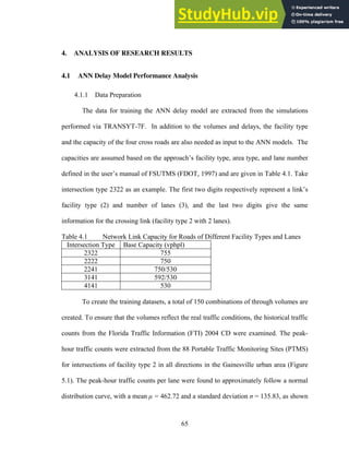
![in Figure 5.2. Therefore, the normal distribution was for intersections of facility type 2
when creating the simulation scenarios. Because no PTMSs are found for undivided
arterials (facility type 3) and local collectors (facility type 4), it is assumed that the peak-
hour traffic for these facility types also follow a similar normal distribution. The µ and σ
are slightly adjusted so that [µ-3σ, µ+3σ] properly contains the assumed base capacities.
This range represents the 99% confidence interval of a normal distribution. In other
words, the volumes selected will fall within this range with a 99% probability. Table 4.2
gives the normal distribution parameters for different intersection types.
Figure 4.1 Locations of 88 PTMS for Divided Arterials in the Gainesville Urban
Area
66](https://image.slidesharecdn.com/astatictrafficassignmentmodelcombinedwithanartificialneuralnetworkdelaymodel-230806163824-28972993/85/A-Static-Traffic-Assignment-Model-Combined-With-An-Artificial-Neural-Network-Delay-Model-80-320.jpg)
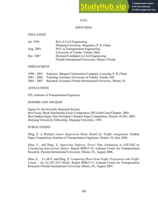
![Figure 4.2 Distribution of Peak-hour Traffic Counts of 88 PTMS for Divided
Arterials
Table 4.2 Normal Distribution Parameters for Volumes by Intersection Type
Intersection Type µ σ
2322 462.72 135.83
2222 462.72 135.83
2241 462.72 135.83
3141 400.00 125.00
4141 400.00 125.00
The 150 combinations of through traffic volumes were created by sampling from
normally distributed volumes within the range of [µ-3σ, µ+3σ] using random numbers.
For all types of intersections in this study, the heaviest through volume simulated was
approximately 1.4 times that of the corresponding approach’s base capacity.
The simulation scenarios also require left-turning volumes. Assuming seven
turning ratios for generating different combinations of turning traffic, which are 10%,
15%, 20%, 25%, 30%, 35%, and 40%, the number of combinations of four turning ratios
is 74
= 2,401. However, because an ANN model does not need to be trained with all
67](https://image.slidesharecdn.com/astatictrafficassignmentmodelcombinedwithanartificialneuralnetworkdelaymodel-230806163824-28972993/85/A-Static-Traffic-Assignment-Model-Combined-With-An-Artificial-Neural-Network-Delay-Model-81-320.jpg)
![possible situations to make predictions, not all of the 2,401 turning ratio combinations
have to be considered in training. It was found that the ANN model did not seem to be
sensitive to small variations of turning ratios under certain through traffic conditions. For
instance, an intersection with a turning ratio combination of [0.1 0.1 0.25 0.3] has no
significantly different traffic situation compared to one with a turning ratio combination
of [0.1 0.1 0.2 0.3] when the four through volumes are fixed. Therefore, only 12 turning
ratio combinations are randomly selected from the 2,401 to combine with the through
volumes and create the ANN training scenarios. The performance of ANN delay models
has proven that this proportion is adequate for the analysis. As a result, there are 1800 (=
150 × 12) scenarios simulated for each intersection. Extracted from these 1800 scenarios
are respectively 7200 (= 1800 × 4 legs) samples for either through or left-turn movements
of each intersection type. During the training of the ANN delay model, the input data are
divided into three groups: training data, validation data, and testing data. All of the
samples are employed to train the ANN delay model except that approximately 15% of
the 7200 samples are randomly allocated to test the ANN delay model’s accuracy at a
later stage. The ANN training employs “supervised learning,” that is, the training process
is simultaneously supervised by the scaled conjugate gradient training algorithm that
applied validating data to the trained ANN to correct potential overfitting. After the
training of the ANN model, the testing data are used to evaluate the ANN model’s
performance.
4.1.2 Evaluation of the ANN Delay Model
The accuracy of the ANN delay model’ delay estimates is an essential condition
to ensure the overall performance of the combined system. Note that there are in fact two
68](https://image.slidesharecdn.com/astatictrafficassignmentmodelcombinedwithanartificialneuralnetworkdelaymodel-230806163824-28972993/85/A-Static-Traffic-Assignment-Model-Combined-With-An-Artificial-Neural-Network-Delay-Model-82-320.jpg)


![Within one iteration of traffic assignment, Tc is provided by the ANN delay model
for every turning movement of an intersection. Based on identification number of
intersections, the ANN delay model is able to determine if Tc is resulted from a delay
estimate for through traffic, right-turn movements, or left-turns. Tl is, on the other hand,
calculated by the Cube traffic assignment model in the form of Bureau of Public Roads
(BPR) volume-delay function using Eq. 4.3:
Tl = tu[1+ k(v/c) m
] Eq 4.3
where
tu = free flow travel time, a constant (undersaturate condition),
k = saturation weight factor (default value, 0.15),
m = saturation power factor, (default value, 4).
The goal of the traffic assignment is to find the minimum total travel cost of the
network:
Eq. 4.4
∑
=
=
n
i
i
T
Z
1
)
min(
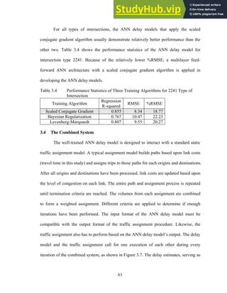
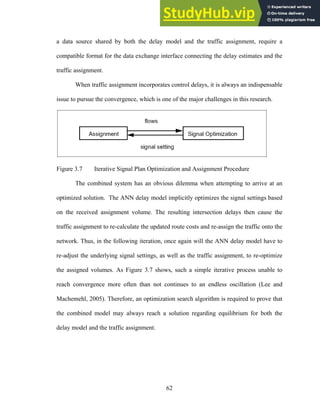
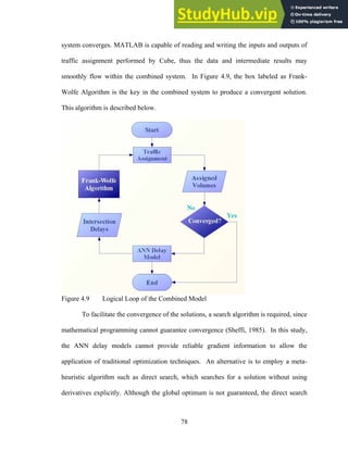
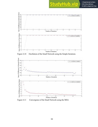
4.3 The Combined System
As mentioned in Chapter 3.3, the combined system of the delay model and traffic
assignment is an iterative process, as illustrated in Figure 4.9. The user equilibrium (UE)
traffic assignment is performed by Cube, which produces link volumes. These link
volumes and turning movements are provided to the ANN delay model, which updates
control delays based on the assigned volumes. These delays are sent back to Cube for the
next run of the traffic assignment. This process repeats until the solution of the combined
77](https://image.slidesharecdn.com/astatictrafficassignmentmodelcombinedwithanartificialneuralnetworkdelaymodel-230806163824-28972993/85/A-Static-Traffic-Assignment-Model-Combined-With-An-Artificial-Neural-Network-Delay-Model-91-320.jpg)

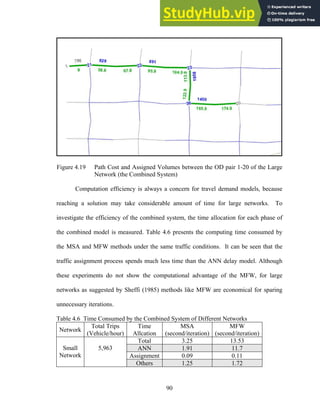


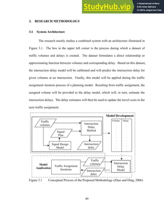
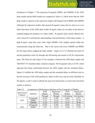
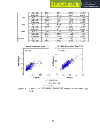
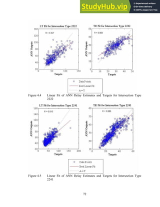
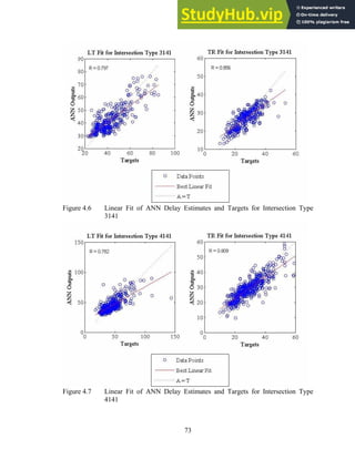
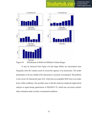
The document discusses the development of a combined system that integrates an artificial neural network (ANN) delay model with a traffic assignment model to estimate intersection delays and route choices simultaneously. The ANN delay model is trained using extensive simulations based on TRANSYT-7F signal optimizations to estimate delays for different intersection types. A combined iterative optimization and assignment procedure is then developed to achieve a convergent traffic assignment solution that considers the interaction between traffic routing and signal controls.