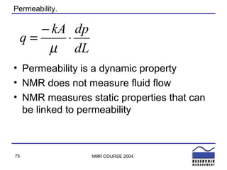
NMR PETROPHYSICS
Class Exercise (NMR Perceptions) The purpose of petrophysics in formation evaluation Primary Objectives Secondary Objectives Nice to have (but almost impossible)
Class Exercise (NMR Perceptions) Based on you conclusions about petrophysics Where does NMR fit in? Primary products Secondary products Might deliver (but unreliable)
Petrophysics Review Porosity Saturation Wettability Surface and Interfacial tension  Capillary pressure Permeability In Tarek Ahmeds ‘Reservoir Engineering Handbook’ the fundamentals of rock properties are The petrophysicists’ primary role is the quantification of these properties, through the evaluation of laboratory and log evaluation.
Petrophysics Log analysis is part of the discipline of petrophysics ‘ A log analyst is a scientist, a magician and a  diplomat…… He has extensive knowledge of geology, geophysics,  sedimentology, petrophysics, mathematics,  chemistry, electrical engineering and economics’ E. R Crain
NMR And Petrophysics NMR is primarily a porosity and fluid characterisation tool Its primary advantage is that NMR porosity is lithology independent and the derivation of porosity requires no correction for matrix properties Secondary Benefits Pore size distribution Fluid characterisation Saturation (clay, capillary, free water and hydrocarbons) Nice to have (but difficult) Wettability Capillary pressure Risky (but possible) Facies or rock typing information
NMR And Permeability Permeability (Holy Grail) NMR does not directly measure permeability, but does provide parameters useful for the calculation for of permeability from empirical equations Porosity, Mean pore size Porosity partitions Clay bound water Capillary bound Free fluid
Porosity (after Hook). The ratio of void (or fluid space) to the bulk volume of rock containing that void space.  Porosity can be expressed as a fraction or percentage of pore volume . 1) Primary porosity refers to the porosity remaining after the sediments have been compacted but without considering changes resulting from subsequent chemical action or flow of waters through the sediments. 2) Secondary porosity is the additional porosity created by chemical changes, dissolution, dolomitization, fissures and fractures. 3) Effective porosity is the interconnected pore volume available to free fluids, excluding isolated pores and pore volume occupied by adsorbed water (the engineers Porosity). 4)  Total Porosity is all the void space in a rock and matrix, whether effective or non effective.  Total porosity includes that porosity in isolated pores, adsorbed water on grain or particle surfaces and associated with clays.
Porosity Definitions TOTAL:  Total void volume. Clay bound water is included in pore volume Not necessarily connected Core analysis disaggregated sample NMR core analysis Density, neutron log (if dry clay parameters used) NMR logs Effective (connected): Void volume contactable by fluids Includes clay bound water in pore volume? Possibly sonic log Effective connected Rock Bulk Volume Rock Matrix Clay Clay bound water Total Porosity Effective Porosity log analysis Capillary bound water Free  water Hydrocarbons Minerals
Porosity Definitions Effective (log analysis): Void volume available for storage of hydrocarbons Includes capillary water Excludes clay bound water in pore volume Unconnected pore volume not necessarily excluded Porosity logging tools if wet clay parameters used Effective connected Rock Bulk Volume Rock Matrix Clay Clay bound water Total Porosity Effective Porosity Log Analysis Capillary bound water Free  water Hydrocarbons Minerals
T2 Model 0.1 1.0 10.0 100.0 1000.0 10000.0 Rock Bulk Volume Rock Matrix Clay Clay bound water Total Porosity Effective Porosity Capillary bound water Free  water Hydrocarbons Minerals T2 cutoff NMR is unique it measures total porosity and can be partitioned into pore-size and fluid component
T2 & Porosity -  Echo Data Underlying CPMG decay CPMG echoes T 2  relaxation (msec) AMPLITUDE Calibrated To porosity At start of sequence Immediately after polarization All ‘fluid’ is polarised = Total Porosity Total porosity
Possible Error in Total Porosity Underlying CPMG decay CPMG echoes First echo (e.g TE = 200 usec) Noise Noise and timing of first echo effects the extrapolation to time = 0
Porosity From T2 Data 0.1 1.0 10.0 100.0 1000.0 10000.0 Inversion to  T2 Distribution of Exponential Decays Porosity is calculated as sum of T2 bins in distribution
Exercise – Calculation of porosity The CMR tool is calibrated using a 100 p.u. signal using a water bottle. CMR porosity is calculated using the  general  equation: Actual equation for the CMR tool :
Calibration of Lab Data A sample reference is used Water bottle partly filled to a known volume Doped with a relaxation agent (to reduce T2) Sometimes doped to reduce signal with D 2 0 (To a specific porosity) Amplitudes are then  compared
Calibration of Logging Tools Shop calibration Calibrated using a special calibration tank Calibrated at well site using bottle of water (100% porosity)
Calibration of Logging Tools (MRIL Example) Pre logging: Calibration tank made of fibre glass, lined with thin metal coating Tank acts as container for water sample and faraday cage to shield unwanted RF Three chambers Outer chamber, water is doped with cupric to reduce relaxation time of water and speed up relaxation Inner chamber filled with brine to simulate bore hole conditions
Pore Size Distributions The NMR measurement measures the relaxation of  proton spins.  Relaxation occurs by three main processes   Assuming the rocks are 100% water saturated relaxation due to  surface relaxation is much faster then bulk relaxation (in the fast diffusion limit).  In a homogenous field diffusion is negligible.  Diffusion is an important process if field gradient of fluid has a high diffusion coefficient The fast diffusion limit is where all the pores are small enough and surface relaxation mechanisms slow enough that a typical molecule crosses the pore many time before relaxation.
Pore Size in 100% Water Saturated rocks Rock Grain Spin diffuses to pore wall where a proton spin has a probability for being relaxed In a porous system filled with a single phase Each pore-size has a characteristic T2 decay constant.  The smaller the pores the faster the relaxation (short or fast T2)
Pore Size in 100% Water Saturated rocks
Pore Size in 100% Water Saturated rocks 0.1 1.0 10.0 100.0 1000.0 10000.0 Rock Bulk Volume Rock Matrix Clay Clay bound water Total Porosity Effective Porosity Capillary bound water Free  water Hydrocarbons Minerals T2 cutoff
Measurement of Relaxivity and Pore Size Pc/r & T2) Pc/r & (k*1/T2) Lab Calibration of Data Relaxivity ( ρ ) is expressed in units um/s
Exercise If  ρ  increases but pore size is constant what happens to the value of T2. If  ρ  increases, what are the implication for the measurement of T2. If  ρ  is low what is the implication for wait time (T1).
Impact of Lithology Lithology and relaxivity Sandstone  ρ e  = 23 um/s Dolomite  ρ e  = 5 um/s Limestone  ρ e  = 3 um/s For example a T2 of 33 msec in sandstones = T2 of  0.033 sec  = pore (throat) size of 0.759 um
Pore Size NOTE: When comparing NMR and capillary pressure, NMR measures surface to volume ratio of the pore and capillary pressure equates to pore throat size. The two are only exactly comparable if the pore systems approaches that of a bundle of tubes. However comparison of NMR and capillary pressure does alllow NMR to be related to pore throat size.
Inversion & Porosity and Pore Size Distribution T 2 x T 2 y T 2 z Exponential decay characterises Pore size Total amplitude characterises pore volume
Inversion T 2 x T 2 y T 2 z T 2 x T 2 y T 2 z T2x, y and z are T2 bins, or if scaled to pore size, pore size bins.  Height of column is  pore volume
T2 Distribution Reflects Porosity ‘Bins’ Porosity is sum of porosity bins (x+y+z) T 2 x T 2 y T 2 z
Inversion quality Control Underlying CPMG trend Fit 1 (good) Fit 2 (poor) T2 (ms) Echo Amplitude RMS Error of Fit Well fitted data with evenly distributed error of fit Poorly fitted data with  systematic variation in error of fit
Demonstration of Inversion LIVE DEMO BASED ON CMR200 Data Echo trains Time domain porosity Inversion Smoothing weight Effect of echo filtering Porosity from T2
The Limitations of Inversion Supplementary Notes Inversion limitation discussion
Fluid effects 100 % Water saturated pores: Surface limited relaxation Pore-size information   Oil in water wet pores: Oil does not see pore wall Bulk relaxation Water sees pore wall Surface limited relaxation Relaxation is a function of film thickness  h   h
Hydrocarbon effect on T2 distribution Hydrocarbon effect on T2 distribution 100% Brine Saturated Water wet with oil Producible water (free fluid) Bound fluid (irreducible water) Producible hydrocarbon (free fluid) Bound fluid (irreducible water) T2 increases since hydrocarbon Is not limited by pore-size T2 is limited by pore size in 100% Sw rocks
Fluid and T2 Relaxation
Bulk Relaxation T2 LM Viscosity (cp) 1 10 100 1000 10000 1 10 100 1000 0 50 100 150 200 0.1 1 10 100 T2 LM secs) water 6 cp oil 20 cp oil Temp (deg C)
Bulk Relaxation Oil and Gas Oil viscosity and T2 (150 degF) Density of gas (150 degF)
Density and diffusion coefficient of gas 150 deg F
Fluid Properties
Fluid Properties Calculator /*convert temp to kelvin temp_k = (0.555556)*(temp_F+459.67) /*calculate Bulk T1 T2 oil, water and gas /*convert to ms since equation for seconds /* MU in cp, density in g/cc, temp in Deg K T12B_OIL = (3*(temp_k/(298*MU_OIL))) * 1000 T12B_WATER = (3*(temp_k/(298*MU_WATER))) * 1000 T12B_GAS =(25000*(RHO_GAS/(temp_k**1.17))) * 1000
Fluid Properties Calculator /*calculate the diffusion coefficents DCO_WATER = ((1.3*temp_k)/(298*MU_WATER))*(10**-5) DCO_OIL =  ((1.3*temp_k)/(298*MU_OIL))*(10**-5) DCO_GAS = (0.085*((temp_k**0.9)/RHO_GAS))*(10**-5) /*Tool Coefficients (TE in MSEC) tco = (C*GMR*G*TE)*(C*GMR*G*TE)
Fluid Properties Calculator t2do = 12 / (tco*DCO_OIL) T2_OIL = 1/((1/t2do) + (1/(T12B_OIL/1000)) ) * 1000 t2dg = 12 / (tco*DCO_GAS) T2_GAS =  1/((1/t2dg) + (1/(T12B_GAS/1000)) ) * 1000
Qualitative Fluid Substitution. Bound fluid = Sw irr 2. Remove free-fluid (water) 3.  Add in free fluid water so that T2LM of free fluid  = T2 predicted for hydrocarbon 1.
Exercise  - Predicting Fluid effects USE 250 deg F, C=1.08, G = 19.1 g/cm and, GMR = 18.1) (TE 0.6 msec)  BRINE 20 cp Oil 6 cp Oil Gas (0.2 g/cc)
Exercise  - Predicting Fluid effects Excercises\Model Answers\Solution Fluid Excercise.ppt
Fluid Typing Basics: Exploit T1 contrasts of fluid Diffusion contrasts fluids Set acquisition parameters  That separate water from hydroocarbons Depends on T1 or diffusion contrasts
Polarization (T1) Contrast T1, amount of time taken to polarize water Requires large T1 contrast Used in gas and light oils (< 5 cp) Best in oils < 1 cp Not suitable for more viscous crude oils Acquistion Two wait times  Long (TWL): polarizes water and hydrocarbons Short (TWS): polarizes water only
Polarization (T1) Contrast Hydrocarbon Typing  Using Polarization Contrasts T1 WATER T1 WATER + OIL + Gas T2 T2 Differential OIL + Gas T2 Time Domain Processing gas oil water water gas oil
Diffusion Contrast Uses diffusion contrast Increased echo spacing shortnes T2 of fluid with high diffusion coefficients Gas application (limited) More viscous oils (medium – high viscosity) Limited success for gas due to difficulty of measuring extremely short T2 of gas at long echo spacing
Diffusion Contrast (medium – high viscosity oils) SHIFTED WATER + OIL WATER + OIL TE=Short: no diffusion TE=long: diffusion Water  shift Hydrocarbon Typing  Using Diffusion Contrasts
Enhanced Diffusion Water has an upper bound for apparent (pore size limited) T2 Vary effectiveness of the diffusion component of water T2 Create a detectable contrast between water and oil Medium viscosity oils
Enhanced Diffusion 0.1 1.0 10 100 10 100 1000 T2 oil T2DW TE = 3.6ms G = 19.1 G/cm T = 200 deg F  Viscosity (cp) Relaxation Time (msec)
Enhanced Diffusion T2DW
Logging Gas Reservoirs NMR porosity will underestimate Total porosity because: The low hydrogen index (tool calibration assume HI = 1.0) Insufficient polarization of gas Density logging overestimates porosity because: Measured formation density is reduced by gas (assuming that fluid density is not corrected for gas) ρ b =  ρ ma (1- Φ +  ρ fl  Φ (1-S g,xo )+  ρ g Φ S g,xo   Φ nmr =  Φ S g,xo  (HI) G  Pol g +   Φ (1-S g,xo )(HI) f
Logging Gas Reservoirs Polariztion function for gas:  Pol g =1-exp (-W/T1g)
DMRP Inputs & Calculated Logs
Logging Gas Reservoirs & Density NMR Porosity (DMRP) In the presence of gas: Density log overestimates porosity (Fluid density deficit) NMR log underestimates porosity (HI index deficit) Providing that the polarization effect is understood, the deficit between the porosity estimates of the two logs is proportional to the gas saturation. This effect can be approximated using the equation: PHIT_DMR = 0.6*PHIA_DEN + 0.4 * PHIT_NMR where: PHIT_DMR = combined density NMR porosity PHIA_DEN = apparent porosity derived from the density log PHIT_NMR = porosity derived from the NMR log Freedman, R., Chanh Cao Minh. Gubelin, G. Freeman, J. J. McGuiness, T. Terry, B. and Rawlence, D. 1998. Combining NMR and Density Logs for Petrophysical Analysis in Gas Bearing Formations . Transactions of the SPWLA 39th Annual Logging Symposium, May 26-29, Keystone Colorado. 1998. Paper II.
Magnetic Resonance Fluid characterization Station log  with  CMR+ Pulse sequences investigate the different  polarization and diffusivity of the fluids.  POLARIZATION SHORT TE BULK & SURFACE  RELAXATION (Short TE) LONG TE DIFFUSION (LONG TE)
Magnetic Resonance Fluid characterization Plot  of T2 v. diffusivity This indicates expected position of fluids in a clean sandstone formation. T2 distribution  (corrected for diffusion) 1 mS 1000 mS 10 -6  m 2 .s -1 10 -11  m 2 .s -1 Water line Oil line Gas Light Oil Heavy Oil Bound Fluid Diffusivity Gas line
Magnetic Resonance Fluid characterization Example of MRF station Align at top corner on each page Consistent image height Image Area Gas  Reservoir oil  Oil Filtrate  Bound  Water
Wettability The tendency of one fluid to spread on to or adhere to a solid surface in the presence of other immiscible fluids Fluids that in molecular contact with a mineral surface have a relaxation time less than the bulk fluid relaxation time This enhanced relaxation is due to surface relaxation phenomena NMR core experiments have been  made to try and qualify wettability
Wettability From NMR Logging, Coates et al .
Bound Fluid Bound Fluid Includes Chemically bound water (crystal lattice water) Adsopbed water (surface) Clay bound water Capillary bound water
Bound Water NMR has the potential to detect Clay bound water Capillary Bound Water
Connate Water Saturation The connate water saturation is defined by capillary bound water, and defined by a finite minimum irreducible water saturation on a capillary pressure curve.
Connate Water Saturation Pc (or h) Water Saturation 0% 100% Pd Swc Pd = Displacement pressure. (minimum capillary pressure required to displace the Wetting phase from the largest  capillary pore Swc = Connate irreducible water saturation
Bound fluid in relation to pore size The average capillary radius: Pore size and T2 relaxation
T2 Cutoffs 0.1 1.0 10.0 100.0 1000.0 10000.0 Rock Bulk Volume Rock Matrix Clay Clay bound water Total Porosity Effective Porosity Capillary bound water Free  water Hydrocarbons Minerals T2 cutoff
T2 Cutoffs T2 is proportional to pore-size T2 cutoff is pore-size cutoff More meaningful as a capillary pressure cutoff T2 cutoffs are a function of Capillary pressure chosen for Swc Choice depends on interpretation Producible water (i.e. capillary pressure) Permeability equation (i.e. pore-size)
Variation In T2 Cutoffs FWL Borehole HAFWL Sw A B A B 100 0 Pc (psia) 480
T2 Cutoff From Capillary Pressure (Mercury) Pc Sh Sandstone  ρ e = 23 um/s σ  for  oil water 22 dynes/cm θ  for oil water = 35 degs σ  for air mercury water 480 dynes/cm θ  for  air mercury  = 140 degs pw=1.0 g/cc phc=0.85 g/cc Lab Data
T2 Cutoff From Capillary Pressure (Mercury) Calculate T2 cutoff at S wc Calculate T2 cutoff  at 100 ft HAFWL Show equivalent Pc on cap pressure curve Calculate Sw  at 100 ft Convert to T2 Exercise
Spectral Bound Fluid Bound flluid resides in: Small pores Pore throats Pore lining Each pore size in the NMR spectra is assumed to contain some bound water The distribution of of bound water is defined by a weighting function.
Spectral Bound Fluid Bound fluid = Capillary bound + Surface film b W = f(T2) Sandstone Model: m = 0.0113; b = 1.
Permeability. Permeability is a dynamic property NMR does not measure fluid flow NMR measures static properties that can be linked to permeability
Permeability. Exercise List properties that NMR measures that can be used to infer permeability? List those properties in order of importance
Permeability and Capillary Pressure Pc (or h) 0% 100% sb & Pc Strong correlation between Capillary pressure curves  and permeability? Critical threshold pore  size and volume
Permeability
Permeability and Pore Size Capillary pressure curves suggest a strong correlation between permeability and: Pore throat size Pore volume NMR measures: pore body size, but in almost all sandstones and some carbonates a correlation exists between pore body size and pore throat size The amount of trapped bound fluid is related to pore throat size The average throat size (pore size) is related to the average T2 value
Permeability Models Two most common models, permeability varies as  Φ 4 . Arbitrary (loosely based on Archie’s explanation of resistivity). Require an additional factor to account for pore throat size. All are based on empirical considerations.
Coates Model The bound fluid term relates NMR pore-size to threshold pore size Problems BFV cannot include hydrocarbons BFV should not be affected by OBM filtrate In gas zones or zones with hydrocarbon that has low hydrogen Index porosity may read too low from NMR log Heavier oils with low T2 may be counted as bound fluid, causing bound fluid to be over-estimated.
The Mean T2 Model (SDR Model) Uses NMR effective porosity T2 is geometric mean of T2 and therefore represent the ‘average’ pore size. Works well in water zones Bulk T2 responses (i.e. hydrocarbon) can skew the response Mean T2 model can fail in hydrocarbon bearing formations.
NMR LOGGING
When Should I Use NMR Logging. Good question, many benefits (and many overheads) Excellent porosity tool Expensive High LIH charges Pore size distributions can be used to quantify petrophysical units Requires calibration Fluid identification Shallow reading tool, logs flushed zone Low resistivty pay Possible applications for permeability prediction Requires extensive core calibration
Primary and secondary objectives Primarily a lithology independent porosity tool, offering great accuracy. Secondarily Fluid typing Pore size distribution Petrophysical facies Permeability
Which tool? The cheapest? CMR High vertical resolution, lower S:N.  Fluid typing requires multiple passes (older generation tools). Pad based eccentred tool (error prone to rugosity) MRIL Lower vertical resolution, higher S:N.  Fluid typing in a single pass Centred tool (error prone to wash-out) Combinability Contracts Regional experience
Which Tool – Basic Tool design Tool specs are continuously changing, for tool sizes and P/T limitations refer to your contractor Next few slides refer to basic differences between tools LWD tools also exist
CMR (e.g. 200) Sensitive region Sensitive region Antenna (rf probe) Magnets
CMR Logging – Single Frequency (CMR 200) Polarization Acquisition (CPMG) TR is controlled by the logging speed
CMR Total Porosity Mode T2 L T WL Phase +ve Phase -ve  Total NE=3000  TOTAL NE = 3000 CPMG=Phase +ve and Phase -ve TE N S N S
CMR Plus Increased logging speed: 30” magnets extend above and below 6” measurement antenna Pre-polarization (prepares the formation) Increased polarization at same logging speed Increased logging speed for same polarization Enhanced precision mode logging Improve resolution at short T2 (i.e. clay bound water)
Enhanced Precision Mode T2 L T WC …… . Single Frequency TE=120ms NE=800 TE=0.6ms, NE=10 repeat*50 TW = 24 s averaging Effective porosity Clay-bound  porosity 4ms-20000ms 0.5ms-2ms = + T WL
Multi-Frequency Tools (e.g. MRIL C & MRIL Prime)
MRIL Prime
Multi Frequency And Depth of Investigation Gradient field, and therfore magnetic field strength is a function of radial distance (r) from the tool surface. Larmor frequency (i.e. frequency of proton oscillation) is proportional to magnetic field strength To detect protons need to select correct frequency band (i.e. radio analogy)
Multi Frequency Tool Selecting a narrow frequency results in a the sensitive volume being a thin cylindrical shell Changing frequency band changes the depth of investigation. Spin tipping only occurs within the tuned frequency band
Multi frequency operation Delta wait time Two different Tw Delta echo spacing Two different TE Increased S:N Multiple acquisitions in different frequency bands
Multi Frequency Acquisition Cycle DTW.
Multi Frequency Tool Advantages Multiple measurement shells  Multiple acquisitions at same depth Improved S:N (more than one measurement at same depth available for signal averaging Multiple experiments – no need for multiple passes for Polarization contrast experiments Diffusion Experiments MRIL C Two Frequency measurements MRIL Prime Multiple frequency measurements One Disadvantage is: Lower resolution
LWD MRIL T1 Saturation Recovery LWD Logging: T2 logging requires rf interrogation field to be stable for duration of T2 experiment (10’s of seconds) Stability is keeping the same sensed volume relative to the rf field generating the CPMG pulses for the duration of the experiment (i.e. sensed volume must be same throughout the experiment). For MRIL measurement shells are  very thin & therefore sensitive to motion.  CMR measurement small cubic sensed volume. Random tool movement during drilling (i.e. vibration) causes instability in magnetic volume. T1 saturation recovery experiments are insensitive to tool motion
LWD MRIL Tool
Saturation Recovery Protons polarised in field 2. Broadband pulse saturates (eliminates) polarisation B 0  Field Protons allowed to recover for Time = t B 0  Field After time = t, some of the protons have recovered Magnetization measured by a very short pulse sequence Time for total recovery = T1
T1 Saturation Recovery Recovery times are stepped between measurements Saturation pulse Measurement pulse Variable delay Delay sequence 1, 3, 10, 30, 100, 300, 1000, 3000 msec
T1 Saturation Data Nuclear polarization 1 0 B 0  exposure time (variable delay) 1 0
T1 Saturation Recovery & Logging The measurement pulse is very short duration (1/2000 sec).  Therefore tool relatively stable in this short time. Magnetic field and saturation pulse cover large volume compared to measurement pulse.  Therefore measurement pulse compared to magnetic field is stable for the short duration of measurement T1 is much longer experiment than T2.  But while drilling this is not a problem LWD T1 (delivers limited spectrum and mainly used for porosity) T2 measured while pulling out of hole for full T2 relaxation
Depth of Investigation MRIL (DOI is radius from tool centre) 6 in tool 200 deg F 14.5 in and 16.5 in (high and low frequency) 8.5 in hole, 16 in DOI corresponds to 3-4 in from borehole wall. 4.5 in tool 10  and 11.5 in CMR (Quoted for CMR 200) 0.5 to 1.5 in CMR and MRIL tools generally reads in the flushed zone
Setting Up Logging Jobs Be clear on the objectives Porosity Bound fluid Fluid typing Etc Parameters Wait time Number of echoes Frequency mode
Job Planning Basic Steps Borehole temperature and pressure Determine NMR fluid properties: Bulk T1 and T2, Diffusion coefficient and HI You will need, viscosity, HI, mud type Expected porosity Decay spectrum, polarization Activation sets and frequency cycling Porosity logging Hydrocarbon logging (DTE, DTW) Clay types (presence) Enhanced precision mode
Job planning additional information NMR core data T1, T2  Capillary pressure data BFV cutoff Conventional core analysis data Porosity and permeability calibration
Pre-logging Checks Correct acquisition mode Hole clean up with ditch magnet recommended with hole debris is suspected Shop calibration checked at well site (if possible) Tool tuning May need to be repeated several times through the logging job.
Pre Logging Checks Acquisition Modes Total porosity Maximise resolution Maximise S:N Fluid Typing Correct mode for expected fluids Light hydrocarbons = Dual Tw Viscous Oil, Dual Te Intermediate oils, Enhanced diffusion Frequency cycling diagram MRF planning (i.e. in MDT program)
Pre Logging Checks Tool Tuning (Example CMR) The tool must be operated at the Lamour frequency, which is determined by the magnetic field strength Magnetic field strength will vary with Formation mineralogy Temperature Hole debris
Tool Tuning, Frequency Sweep Conducted Down hole over a porous zone Tuned 3 times (1) Repeat pass, (2) Before Main Pass (3)After logging Ensure temperature stabilization Tool is moved slowly up and down Used to determine operating frequency Tool is retuned if changes in magnetic field gradient occur (change in Delta Bo)
Tool Tuning, Frequency Sweep Signal Amplitude Frequency Lab calibration Result of sweep down hole
Implications of Poor Tool Tuning Signal amplitudes will be low, compared with the porosity calibration Shape of T2 distribution not effected Porosities will be low Errors in frequency and  porosity 1 kHZ -0.2% low 3 kHZ -1.5% low 5 kHZ -3.4% low
Log Quality Control 4 steps Check acquisition parameters against job plan Tool behaviour Tool tuning plots Noise evaluation Compare raw and processed data (i.e. pre and post stack) Get Log QC plot
Log Quality Control Guidelines - CMR Key parameters are: Gain Delta B 0 Signal Phase Noise standard deviation Gamma regularization MORE IN PRACTICAL NMR LOG INTERPRETATION
Log Quality Control Guidelines - MRIL  Key Parameters are: Gain and Q level B1 and B1 nod Chi Noise indicators Offset Noise Ringing IENoise Low and High Voltage sensors Phase correction information (PHER, PHNO and PHCO) Temperature MORE IN PRACTICAL NMR LOG INTERPRETATION
PRACTICAL NMR LOG EVLAUTAION
General Work Flow Evaluate raw data QC checks Porosity calibration checks Echo data processing Inversion Porosity calculation Cross check with other logs Evaluate T2 distributions Fluid typing Multi acquisition processing Bound and free fluid T2 cutoff Spectral Bissecting Clay bound water Permeability Rock Typing Capillary pressure conversion Specialist Activities Core  Calibration Forward  Modelling Log Analyst / Interpreter
Practical NMR Log Processing: CMR CMR quality control Porosity calibration CPMG processing Phase angle Phase rotation Data stacking Inversion
CMR Quality Control - GAIN Gain: Amount of loading applied to the tools circuits by fluids and formation Gain is the amount amplitude of the signal received by the RF antenna Gain is frequency dependent, and optimum gain depends on correct tool tuning Gain should not Have sudden changes or spikes be 0 Drop below 0.3
CMR Quality Control – Delta B 0 Delta B o Estimated by the hall probe and temperature sensor Difference between two is Delta B 0 Indicates amount of debris on on magnets If it exceeds 0.1 mtesla. The tool should be retuned
CMR Quality Control, Signal Phase The phase angle is used to extract the signal amplitude and signal noise from the x and ycomponents to generate the echo-train data used for inversion to T2 distributions. In porous intervals, the signal phase should remain relatively stable (±100). In low porosity In shaly zones, signal noise is difficult to estimate due to low signal to noise. Consequently, the Signal phase should only be examined with respect to log quality in clean porous intervals. Signal Phase Calculation Explained in CMR processing
CMR Quality Control (Polarisation Correction) Older tools only where Tw < 3*T1 of formation & fluids. As the tool is pulled past the formation, the formation experiences a time dependent magnetic field (wait time) and thus time dependent polarization.  For the CMR 200, at speeds higher than 5 cm/s there is a significant loss in polarization for fluids with a T1 greater than 1s. Consequently, at logging speeds greater than 5 cm/s there is a significant loss of polarization For fluids and large pores with long T1's. Since porosity is calculated as the sum of the amplitudes of the T2 distribution multiplied by the CMR calibration value, the porosity estimated from CMR data is affected by the polarization correction.
CMR Quality Control (Polarisation Correction) Analogue Model Inversion Fluid Sub Tw = 1 sec Lost porosity With Tw = 1 sec
CMR Quality Control (Polarisation Correction) The polarization correction is
CMR Quality Control (Polarisation Correction) As part of the quality control checks, three different porosity estimates are calculated usingthree different T1:T2 ratios (R). The default values taken for R are 1, 1.5 and 3.  ERRMINUS and ERRPLUS are the differences between the default and limit values for R The CMR log can be checked for incomplete polarization (insufficient wait time) by comparing the three different porosity estimates calculated using the three different values of R. Where theformation has been subject to a sufficient wait time, and complete polarization has occurred,there should be no difference in porosity calculated using different wait times. In cases wherethe wait time was insufficient for complete polarization, porosities will differ over the range ofT1:T2 ratios selected.  Insufficient wait time is normally flagged when the difference between porosity calculated using the minimum R and maximum R is greater than 2 p.u. (WAIT_FLAG)
Quality Control of CMR data Signal-to-Noise The Raw CPMG data is inherently noisy The S:N is acceptable if distributed evenly across the Echo train S:N can be increased by data stacking S:N can be expressed as RMS noise or a S:N ratio
Quality Control of CMR data Signal-to-Noise Good data
Quality Control of CMR data Signal-to-Noise Noisy  Data
Quality Control of CMR Gamma Gamma A regularization method is used to generate a smooth T2 distribution.  For Schlumberger processed CMR data Gamma controls the amount of smoothing Gamma depends on the S:N, in high S:N environments (high porosity) Gamma is usually less than 5.  In low SLN environments Gamma is more than 10.
CMR QC plots
CMR Porosity Calibration. Alternatively CMR porosity can be calibrated directly to another measurement (i.e. core data).
CPMG (Echo) Processing CPMG data is collected using a quadrate detection system in which the signal is recorded in two channels (R and X). The R and X data is used to estimate the phase of the signal and the two channels are combined to generate (1) a phase coherent channel that contains the signal, and (2) a noise channel. Echo R Echo X Phase Angle signal noise
CPMG (Echo) Processing The phase angle is calculated as: where φ = phase angle i  =  ith  echo of the echo train k  = number of echoes to be used in the phase angle calculation
CPMG (Echo) Processing R and X = inphase and quadrature detected component of the CPMG The CPMG signal and noise is calculated by rotating the channel data through the phase angle . signali = Ri *cos  φ  + Xi * sin  φ noisei = Ri *sin  φ  - Xi *cos  φ   where: signali  = signal of the  ith  echo noisei  = noise of the  ith  echo Ri = inphase component of the  ith  echo Xi = quadrature component of the  ith  echo
S:N and Vertical Resolution (data stacking) 8 Level Stack Stack Base to Top
S:N and Vertical Resolution (data stacking) Demonstration
Practical NMR Log Processing: MRIL. Multi-Phase & Frequency Processing
Practical NMR Log Processing: MRIL. Raw data on time-based file Apply running average (minimum stack) Phase angle and phase rotation Environmental corrections Time to depth conversion
Practical NMR Log Processing: MRIL.  DTE DATA Frequency 1 Frequency 2 Frequency 3 Frequency 4 md time Running Average = 8 (PAP * NF) Phase Alternated Pairs PAP’s .
Practical NMR Log Processing: Data Coding
MRIL Running averages & Minimum Running Average Running Average (RA) Stack several echo trains to improve S:N  Data is collected in phase alternated pairs Data is collected over several frequencies (depending on acqusition mode) Minimum Running Average Similar data is gathered together over the acquistion cycle.  Minimum RA is Number of frequencies * 2 For example DTE uses 4 frequencies.  The sort TE data is collected over 2 frequencies The Long TE is collected over 2 frequencies The minimum RA is 4 for the short and long TE data The running average can be increased to imrove S:N but must be a multiple of the minimum RA
MRIL Running averages & Minimum Running Average DTE data Minimum RA = 4  RA = 16 NOTE RA always in  Direction of time (not depth) Q? In which direction was This data logged, up or  Down? md time
MRIL Phase Rotation Identical technique used for processing CMR data CPMG data is collected using a quadrate detection system in which the signal is recorded in two channels (R and X). The R and X data is used to estimate the phase of the signal and the two channels are combined to generate (1) a phase coherent channel that contains the signal, and (2) a noise channel. Echo R Echo X Phase Angle signal noise
Time Based Data and Depth Conversion Raw MRIL data on time based file After processing the data, the data is converted to depth by sampling the data Time to depth conversion can only be done after the minimum running average has been applied. Time to depth conversion can be carried out: Post minimum RA (Real and Imaginary Data) After phase rotation (ECHO and NOISE) After environmental correction After inversion
Time Based Data and Depth Conversion
Environmental Corrections
Environmental Corrections Salinity Correction The salinity correction is only applied if the Rmf < 10 ohm.m at 75° C. The correction compensates from the loss of hydrogen atoms replaced by salt ions. Temperature Corrections Temperature affects the thermal relaxation of protons and reduces the amplitude of the returned signal. The temperature correction should always be applied. Hydrogen Depletion Correction Increased temperature of the formation reduces the density of the formation fluid and decreases the hydrogen index. Higher pressures increase the hydrogen index. This effect is compensated for by using a Hydrogen Depletion Multiplier, which is a function of porosity and temperature. Environmental corrections are applied during phase rotation of the real and imaginary data.
MRIL Quality Control Gain and Q level B 1  and B 1mod Chi Noise Indicators Offset Noise Ringing IENoise Low voltage sensors High voltage sensors Phase Correction Information
Gain And Q Level Gain is dependent upon the loading of the MRIL transmitter coil by borehole fluids and the formation, and is measured continuously throughout logging. Gain is also frequency dependent, and generally, the operating frequency is chosen to achieve the maximum gain.Gain should be constant; spiking usually indicates tool problems. Q Level  is an estimate of coil quality; certain MRIL activations are designed to run at agiven Q Level (high, medium or low). Q Level depends on the Gain.
Gain And Q Level
B1 Field (B 1  and B 1mod ) The B1 Field is responsible for generating the pulse sequence that is used to acquire the CPMG sequence. With every pulse sequence, the B1 is measured using a test coil.  The B1 Field should remain relatively constant but should show some variation with changes inconductivity and gain. Consequently, the B1 Field should be checked for overall variation andvariation with conductivity and gain.
Chi Equivalent to gamma used in CMR inversion of T2 data. A regularization method is used to generate a smooth T2 distribution Chi limits Mo less than 2, except in low Q situations
Noise Indicators
Noise Indicators High Q Med Q Low Q
Voltage Sensors
Phase Angle Corrections PHER Mean of the noise channel, and should be close to zero, less than 1 for good quality data PHNO Standard deviation of the noise channel, should be comparable in magnitude with other noise indicators PHCO Phase correction angle, should be relative constant in porous intervals (high Q environment), random variation in Low Q (i.e. shales)
T2 Analysis Work Flows
T2 Analysis Work Flows The T2 analysis tool kit Porosity calculation. Denisty NMR Porosity calculation. Estimatation of the T2 geometric mean (T2LM). Calculation of the bound fluid. Estimation of T2 bumps. Permeability. Tracking the T2 of the modes of the distribution (Peak Tracking). Calculation of viscosity.
Porosity Calibrated as previously discussed May be calibrated against core data Calculated from the sum of the amplitudes of the T2 distribution Represents total porosity, including capillary and clay bound water
Porosity
Polarisation Correction The polarization correction is
Polarisation Correction
Porosity Log
T2 Attributes Geometric mean Number of peaks Peak(s) position Ratio of volume under peaks Bound Fluid Free Fluid Clay Bound Water Skewness Kurtosis Principal Components etc
Bound Fluid 0.1 1.0 10.0 100.0 1000.0 10000.0 Rock Bulk Volume Rock Matrix Clay Clay bound water Total Porosity Effective Porosity Capillary bound water Free  water Hydrocarbons Minerals T2 cutoff
Bound Fluid
Spectral Analysis Bound fluid = Capillary bound + Surface film b W = f(T2) Carbonate Model: m = 0.0113; b = 1.  Sandstones m = 0.0618, b = 1.
Bisecting Method. ‘ saddle point’
Permeability
Lab Calibration of NMR data
Lab Calibration Calibration Lab NMR data for Porosity T2 cutoffs Capillary Pressure Data T2 cutoffs Pore size Forward Modelling Reconfiguring lab data for log response Fluid substitution Optimising inversion
T2 Cutoffs 0 0.1 0.1 1.0 10 100 1000 10000 T2 (ms) Por (p.u.) Sw irr  (core) T2 Cutoff 0.1 1.0 10 100 1000 10000 0 1.0 0.8 0.4 0.6 0.2 Porosity Deviation (Frac) BFV Cutoff T2 (ms)
T2 cutoffs 0.1 1.0 10 100 1000 10000 0 1.0 0.8 0.4 0.6 0.2 Porosity Deviation (Frac) T2 cutoff  (ms) Multiple Samples T2 cutoff range
T2 cutoffs 0.1 1.0 10 100 1000 10000 0 1.0 0.8 0.4 0.6 0.2 Porosity Deviation (Frac) RMS average 9.3ms RMS Error Plot Error Associated with single value T2 cutoff
Forward Modelling Predict fluid properties of hydrocarbon Calculate bound fluid T2 cutoff Spectral Bound Fluid Use core calibration (i.e. porous plate de-saturation) Remove free fluid from T2 distribution Substitute in ‘hydrocarbon’ with bulk properties Model raw data
Forward Modelling Spectral bound fluid = Swirr 2. Remove free-fluid (water) 3.  Add in free fluid water so that T2LM of free fluid  = T2 predicted for hydrocarbon 1.
Forward Modelling : Optimising Inversion of Log Data Inversion: SVD T1 min = 0.3 T2 max = 3000 No Bins = 30 T2 maximum is not long enough to capture Long T2 associated with carbonate Analogue Model Inversion
Forward Modelling : Optimising Inversion of Log Data Inversion: SVD T1 min = 5 T2 max = 5000 No Bins = 30 Analogue Model Inversion New bin range better captures the full T2 spectrum
Forward Modelling : Fluid Substitution 3 CP Oil T2 = 1130 msec (150 deg F) Analogue Model Inversion Fluid Sub
Forward Modelling :  Decreased Wait Time (1 sec) Analogue Model Inversion Fluid Sub Tw = 1 sec Lost porosity With Tw = 1 sec
ADDED VALUE FROM NMR
Other Applications NMR facies analysis and flow unit identification Non parametric & statistical techniques Capillary pressure from NMR Pseudo water saturated T2 Capillary pressure conversion Saturation height modelling
NMR Facies ‘ A set of similar NMR T2 distributions that summarise the petrophysical characterics of the rock’ Walsgrove Stromberg and Lowden 1997 ‘ Categorization of types that are recognisable away from the core point allow the extrapolation of petrophysical parameters and interpretation models.’
Facies Analysis ft 0 50 100 150 Porosity Permeability Porosity Permeability Porosity Permeability
Cluster Analysis Distance Coefficient Distance Cutoff
Facimage Examples Facimage
Example 1. Using Analogue Data Log Data Analogue 5 4 3 2 1 Shale Meander Point-bar Braided 0.1 1 10 100 1000 10000 0.1 1 10 100 1000 10000 0.1 1 10 100 1000 10000 0.1 1 10 100 1000 10000 0.1 1 10 100 1000 10000 0.1 1 10 100 1000 10000 0.1 1 10 100 1000 10000
Example 1. Analogue Data Log Data 5 4 3 2 1 Shale Analogue Low K < 100 mD High K > 100 mD 0.1 1 10 100 1000 10000 0.1 1 10 100 1000 10000 0.1 1 10 100 1000 10000 0.1 1 10 100 1000 10000 0.1 1 10 100 1000 10000 0.1 1 10 100 1000 10000
Interpretation from Analogues GR CMRP BFV Permeability T2 Dist Meander Meander Braided Point-bar Low K Model 1 High K Model 2 0  GAPI  150 0.5  V/V  0 0  mD  10000
Capillary Pressure Modelling
Scaling T2 to Pc Pc & k*(1/T2) Pc & k*(1/T2) Pc = K*(1/T2) NMR PC Sw 100000 0 100000 0 0 1 Sw 100000 0 0 1 Pc (height)
Example Ghadames Basin Sh (1-Sw) PC (h)
Rocks With Sw < 1 (i.e. dual phase T2) Rocks with hydrocarbons: T2 influenced by hydrocarbons Fluid substitution to construct psuedo 100% Sw T2 distribution Method only exists for sandstones at present Method: Calculate Swirr (using SBFV method) Predict theoretical T2LM in water wet sandstones Remove free fluid part of spectrum using SBFV method Add in water spectrum such that T2LM = theoretical T2LM
T2LM in Sandstones (from sandstone rock catalogue) Log10(1-Swirr/Swirr) T2LM Yakov Volokitin, Wim Looyestijn, Walter Slijkerman, Jan Hofman. 1999.  Constructing capillary pressure curves from NMR log data in the presence of hydrocarbons . Transactions of the Fortieth Annual Logging Symposium, Oslo, Norway, 1999. Paper KKK 10**(0.772*(LOG10((-1-SWirr)/SWirr))+k K = 1.5
Pseudo 100% Sw T2 Spectral bound fluid = Swirr 1. 2. Remove free-fluid (hydrocarbon) T2LM =10**(0.772*(LOG10((-1-SWirr)/SWirr))+k K = 1.5 3.  Predict   T2LM Add in free fluid water so that T2LM = predicted  T2LM  4.

Nmr Course

  • 1.
  • 2.
    Class Exercise (NMRPerceptions) The purpose of petrophysics in formation evaluation Primary Objectives Secondary Objectives Nice to have (but almost impossible)
  • 3.
    Class Exercise (NMRPerceptions) Based on you conclusions about petrophysics Where does NMR fit in? Primary products Secondary products Might deliver (but unreliable)
  • 4.
    Petrophysics Review PorositySaturation Wettability Surface and Interfacial tension Capillary pressure Permeability In Tarek Ahmeds ‘Reservoir Engineering Handbook’ the fundamentals of rock properties are The petrophysicists’ primary role is the quantification of these properties, through the evaluation of laboratory and log evaluation.
  • 5.
    Petrophysics Log analysisis part of the discipline of petrophysics ‘ A log analyst is a scientist, a magician and a diplomat…… He has extensive knowledge of geology, geophysics, sedimentology, petrophysics, mathematics, chemistry, electrical engineering and economics’ E. R Crain
  • 6.
    NMR And PetrophysicsNMR is primarily a porosity and fluid characterisation tool Its primary advantage is that NMR porosity is lithology independent and the derivation of porosity requires no correction for matrix properties Secondary Benefits Pore size distribution Fluid characterisation Saturation (clay, capillary, free water and hydrocarbons) Nice to have (but difficult) Wettability Capillary pressure Risky (but possible) Facies or rock typing information
  • 7.
    NMR And PermeabilityPermeability (Holy Grail) NMR does not directly measure permeability, but does provide parameters useful for the calculation for of permeability from empirical equations Porosity, Mean pore size Porosity partitions Clay bound water Capillary bound Free fluid
  • 8.
    Porosity (after Hook).The ratio of void (or fluid space) to the bulk volume of rock containing that void space. Porosity can be expressed as a fraction or percentage of pore volume . 1) Primary porosity refers to the porosity remaining after the sediments have been compacted but without considering changes resulting from subsequent chemical action or flow of waters through the sediments. 2) Secondary porosity is the additional porosity created by chemical changes, dissolution, dolomitization, fissures and fractures. 3) Effective porosity is the interconnected pore volume available to free fluids, excluding isolated pores and pore volume occupied by adsorbed water (the engineers Porosity). 4) Total Porosity is all the void space in a rock and matrix, whether effective or non effective. Total porosity includes that porosity in isolated pores, adsorbed water on grain or particle surfaces and associated with clays.
  • 9.
    Porosity Definitions TOTAL: Total void volume. Clay bound water is included in pore volume Not necessarily connected Core analysis disaggregated sample NMR core analysis Density, neutron log (if dry clay parameters used) NMR logs Effective (connected): Void volume contactable by fluids Includes clay bound water in pore volume? Possibly sonic log Effective connected Rock Bulk Volume Rock Matrix Clay Clay bound water Total Porosity Effective Porosity log analysis Capillary bound water Free water Hydrocarbons Minerals
  • 10.
    Porosity Definitions Effective(log analysis): Void volume available for storage of hydrocarbons Includes capillary water Excludes clay bound water in pore volume Unconnected pore volume not necessarily excluded Porosity logging tools if wet clay parameters used Effective connected Rock Bulk Volume Rock Matrix Clay Clay bound water Total Porosity Effective Porosity Log Analysis Capillary bound water Free water Hydrocarbons Minerals
  • 11.
    T2 Model 0.11.0 10.0 100.0 1000.0 10000.0 Rock Bulk Volume Rock Matrix Clay Clay bound water Total Porosity Effective Porosity Capillary bound water Free water Hydrocarbons Minerals T2 cutoff NMR is unique it measures total porosity and can be partitioned into pore-size and fluid component
  • 12.
    T2 & Porosity- Echo Data Underlying CPMG decay CPMG echoes T 2 relaxation (msec) AMPLITUDE Calibrated To porosity At start of sequence Immediately after polarization All ‘fluid’ is polarised = Total Porosity Total porosity
  • 13.
    Possible Error inTotal Porosity Underlying CPMG decay CPMG echoes First echo (e.g TE = 200 usec) Noise Noise and timing of first echo effects the extrapolation to time = 0
  • 14.
    Porosity From T2Data 0.1 1.0 10.0 100.0 1000.0 10000.0 Inversion to T2 Distribution of Exponential Decays Porosity is calculated as sum of T2 bins in distribution
  • 15.
    Exercise – Calculationof porosity The CMR tool is calibrated using a 100 p.u. signal using a water bottle. CMR porosity is calculated using the general equation: Actual equation for the CMR tool :
  • 16.
    Calibration of LabData A sample reference is used Water bottle partly filled to a known volume Doped with a relaxation agent (to reduce T2) Sometimes doped to reduce signal with D 2 0 (To a specific porosity) Amplitudes are then compared
  • 17.
    Calibration of LoggingTools Shop calibration Calibrated using a special calibration tank Calibrated at well site using bottle of water (100% porosity)
  • 18.
    Calibration of LoggingTools (MRIL Example) Pre logging: Calibration tank made of fibre glass, lined with thin metal coating Tank acts as container for water sample and faraday cage to shield unwanted RF Three chambers Outer chamber, water is doped with cupric to reduce relaxation time of water and speed up relaxation Inner chamber filled with brine to simulate bore hole conditions
  • 19.
    Pore Size DistributionsThe NMR measurement measures the relaxation of proton spins. Relaxation occurs by three main processes Assuming the rocks are 100% water saturated relaxation due to surface relaxation is much faster then bulk relaxation (in the fast diffusion limit). In a homogenous field diffusion is negligible. Diffusion is an important process if field gradient of fluid has a high diffusion coefficient The fast diffusion limit is where all the pores are small enough and surface relaxation mechanisms slow enough that a typical molecule crosses the pore many time before relaxation.
  • 20.
    Pore Size in100% Water Saturated rocks Rock Grain Spin diffuses to pore wall where a proton spin has a probability for being relaxed In a porous system filled with a single phase Each pore-size has a characteristic T2 decay constant. The smaller the pores the faster the relaxation (short or fast T2)
  • 21.
    Pore Size in100% Water Saturated rocks
  • 22.
    Pore Size in100% Water Saturated rocks 0.1 1.0 10.0 100.0 1000.0 10000.0 Rock Bulk Volume Rock Matrix Clay Clay bound water Total Porosity Effective Porosity Capillary bound water Free water Hydrocarbons Minerals T2 cutoff
  • 23.
    Measurement of Relaxivityand Pore Size Pc/r & T2) Pc/r & (k*1/T2) Lab Calibration of Data Relaxivity ( ρ ) is expressed in units um/s
  • 24.
    Exercise If ρ increases but pore size is constant what happens to the value of T2. If ρ increases, what are the implication for the measurement of T2. If ρ is low what is the implication for wait time (T1).
  • 25.
    Impact of LithologyLithology and relaxivity Sandstone ρ e = 23 um/s Dolomite ρ e = 5 um/s Limestone ρ e = 3 um/s For example a T2 of 33 msec in sandstones = T2 of 0.033 sec = pore (throat) size of 0.759 um
  • 26.
    Pore Size NOTE:When comparing NMR and capillary pressure, NMR measures surface to volume ratio of the pore and capillary pressure equates to pore throat size. The two are only exactly comparable if the pore systems approaches that of a bundle of tubes. However comparison of NMR and capillary pressure does alllow NMR to be related to pore throat size.
  • 27.
    Inversion & Porosityand Pore Size Distribution T 2 x T 2 y T 2 z Exponential decay characterises Pore size Total amplitude characterises pore volume
  • 28.
    Inversion T 2x T 2 y T 2 z T 2 x T 2 y T 2 z T2x, y and z are T2 bins, or if scaled to pore size, pore size bins. Height of column is pore volume
  • 29.
    T2 Distribution ReflectsPorosity ‘Bins’ Porosity is sum of porosity bins (x+y+z) T 2 x T 2 y T 2 z
  • 30.
    Inversion quality ControlUnderlying CPMG trend Fit 1 (good) Fit 2 (poor) T2 (ms) Echo Amplitude RMS Error of Fit Well fitted data with evenly distributed error of fit Poorly fitted data with systematic variation in error of fit
  • 31.
    Demonstration of InversionLIVE DEMO BASED ON CMR200 Data Echo trains Time domain porosity Inversion Smoothing weight Effect of echo filtering Porosity from T2
  • 32.
    The Limitations ofInversion Supplementary Notes Inversion limitation discussion
  • 33.
    Fluid effects 100% Water saturated pores: Surface limited relaxation Pore-size information Oil in water wet pores: Oil does not see pore wall Bulk relaxation Water sees pore wall Surface limited relaxation Relaxation is a function of film thickness h h
  • 34.
    Hydrocarbon effect onT2 distribution Hydrocarbon effect on T2 distribution 100% Brine Saturated Water wet with oil Producible water (free fluid) Bound fluid (irreducible water) Producible hydrocarbon (free fluid) Bound fluid (irreducible water) T2 increases since hydrocarbon Is not limited by pore-size T2 is limited by pore size in 100% Sw rocks
  • 35.
    Fluid and T2Relaxation
  • 36.
    Bulk Relaxation T2LM Viscosity (cp) 1 10 100 1000 10000 1 10 100 1000 0 50 100 150 200 0.1 1 10 100 T2 LM secs) water 6 cp oil 20 cp oil Temp (deg C)
  • 37.
    Bulk Relaxation Oiland Gas Oil viscosity and T2 (150 degF) Density of gas (150 degF)
  • 38.
    Density and diffusioncoefficient of gas 150 deg F
  • 39.
  • 40.
    Fluid Properties Calculator/*convert temp to kelvin temp_k = (0.555556)*(temp_F+459.67) /*calculate Bulk T1 T2 oil, water and gas /*convert to ms since equation for seconds /* MU in cp, density in g/cc, temp in Deg K T12B_OIL = (3*(temp_k/(298*MU_OIL))) * 1000 T12B_WATER = (3*(temp_k/(298*MU_WATER))) * 1000 T12B_GAS =(25000*(RHO_GAS/(temp_k**1.17))) * 1000
  • 41.
    Fluid Properties Calculator/*calculate the diffusion coefficents DCO_WATER = ((1.3*temp_k)/(298*MU_WATER))*(10**-5) DCO_OIL = ((1.3*temp_k)/(298*MU_OIL))*(10**-5) DCO_GAS = (0.085*((temp_k**0.9)/RHO_GAS))*(10**-5) /*Tool Coefficients (TE in MSEC) tco = (C*GMR*G*TE)*(C*GMR*G*TE)
  • 42.
    Fluid Properties Calculatort2do = 12 / (tco*DCO_OIL) T2_OIL = 1/((1/t2do) + (1/(T12B_OIL/1000)) ) * 1000 t2dg = 12 / (tco*DCO_GAS) T2_GAS = 1/((1/t2dg) + (1/(T12B_GAS/1000)) ) * 1000
  • 43.
    Qualitative Fluid Substitution.Bound fluid = Sw irr 2. Remove free-fluid (water) 3. Add in free fluid water so that T2LM of free fluid = T2 predicted for hydrocarbon 1.
  • 44.
    Exercise -Predicting Fluid effects USE 250 deg F, C=1.08, G = 19.1 g/cm and, GMR = 18.1) (TE 0.6 msec) BRINE 20 cp Oil 6 cp Oil Gas (0.2 g/cc)
  • 45.
    Exercise -Predicting Fluid effects Excercises\Model Answers\Solution Fluid Excercise.ppt
  • 46.
    Fluid Typing Basics:Exploit T1 contrasts of fluid Diffusion contrasts fluids Set acquisition parameters That separate water from hydroocarbons Depends on T1 or diffusion contrasts
  • 47.
    Polarization (T1) ContrastT1, amount of time taken to polarize water Requires large T1 contrast Used in gas and light oils (< 5 cp) Best in oils < 1 cp Not suitable for more viscous crude oils Acquistion Two wait times Long (TWL): polarizes water and hydrocarbons Short (TWS): polarizes water only
  • 48.
    Polarization (T1) ContrastHydrocarbon Typing Using Polarization Contrasts T1 WATER T1 WATER + OIL + Gas T2 T2 Differential OIL + Gas T2 Time Domain Processing gas oil water water gas oil
  • 49.
    Diffusion Contrast Usesdiffusion contrast Increased echo spacing shortnes T2 of fluid with high diffusion coefficients Gas application (limited) More viscous oils (medium – high viscosity) Limited success for gas due to difficulty of measuring extremely short T2 of gas at long echo spacing
  • 50.
    Diffusion Contrast (medium– high viscosity oils) SHIFTED WATER + OIL WATER + OIL TE=Short: no diffusion TE=long: diffusion Water shift Hydrocarbon Typing Using Diffusion Contrasts
  • 51.
    Enhanced Diffusion Waterhas an upper bound for apparent (pore size limited) T2 Vary effectiveness of the diffusion component of water T2 Create a detectable contrast between water and oil Medium viscosity oils
  • 52.
    Enhanced Diffusion 0.11.0 10 100 10 100 1000 T2 oil T2DW TE = 3.6ms G = 19.1 G/cm T = 200 deg F Viscosity (cp) Relaxation Time (msec)
  • 53.
  • 54.
    Logging Gas ReservoirsNMR porosity will underestimate Total porosity because: The low hydrogen index (tool calibration assume HI = 1.0) Insufficient polarization of gas Density logging overestimates porosity because: Measured formation density is reduced by gas (assuming that fluid density is not corrected for gas) ρ b = ρ ma (1- Φ + ρ fl Φ (1-S g,xo )+ ρ g Φ S g,xo Φ nmr = Φ S g,xo (HI) G Pol g + Φ (1-S g,xo )(HI) f
  • 55.
    Logging Gas ReservoirsPolariztion function for gas: Pol g =1-exp (-W/T1g)
  • 56.
    DMRP Inputs &Calculated Logs
  • 57.
    Logging Gas Reservoirs& Density NMR Porosity (DMRP) In the presence of gas: Density log overestimates porosity (Fluid density deficit) NMR log underestimates porosity (HI index deficit) Providing that the polarization effect is understood, the deficit between the porosity estimates of the two logs is proportional to the gas saturation. This effect can be approximated using the equation: PHIT_DMR = 0.6*PHIA_DEN + 0.4 * PHIT_NMR where: PHIT_DMR = combined density NMR porosity PHIA_DEN = apparent porosity derived from the density log PHIT_NMR = porosity derived from the NMR log Freedman, R., Chanh Cao Minh. Gubelin, G. Freeman, J. J. McGuiness, T. Terry, B. and Rawlence, D. 1998. Combining NMR and Density Logs for Petrophysical Analysis in Gas Bearing Formations . Transactions of the SPWLA 39th Annual Logging Symposium, May 26-29, Keystone Colorado. 1998. Paper II.
  • 58.
    Magnetic Resonance Fluidcharacterization Station log with CMR+ Pulse sequences investigate the different polarization and diffusivity of the fluids.  POLARIZATION SHORT TE BULK & SURFACE RELAXATION (Short TE) LONG TE DIFFUSION (LONG TE)
  • 59.
    Magnetic Resonance Fluidcharacterization Plot of T2 v. diffusivity This indicates expected position of fluids in a clean sandstone formation. T2 distribution (corrected for diffusion) 1 mS 1000 mS 10 -6 m 2 .s -1 10 -11 m 2 .s -1 Water line Oil line Gas Light Oil Heavy Oil Bound Fluid Diffusivity Gas line
  • 60.
    Magnetic Resonance Fluidcharacterization Example of MRF station Align at top corner on each page Consistent image height Image Area Gas Reservoir oil Oil Filtrate Bound Water
  • 61.
    Wettability The tendencyof one fluid to spread on to or adhere to a solid surface in the presence of other immiscible fluids Fluids that in molecular contact with a mineral surface have a relaxation time less than the bulk fluid relaxation time This enhanced relaxation is due to surface relaxation phenomena NMR core experiments have been made to try and qualify wettability
  • 62.
    Wettability From NMRLogging, Coates et al .
  • 63.
    Bound Fluid BoundFluid Includes Chemically bound water (crystal lattice water) Adsopbed water (surface) Clay bound water Capillary bound water
  • 64.
    Bound Water NMRhas the potential to detect Clay bound water Capillary Bound Water
  • 65.
    Connate Water SaturationThe connate water saturation is defined by capillary bound water, and defined by a finite minimum irreducible water saturation on a capillary pressure curve.
  • 66.
    Connate Water SaturationPc (or h) Water Saturation 0% 100% Pd Swc Pd = Displacement pressure. (minimum capillary pressure required to displace the Wetting phase from the largest capillary pore Swc = Connate irreducible water saturation
  • 67.
    Bound fluid inrelation to pore size The average capillary radius: Pore size and T2 relaxation
  • 68.
    T2 Cutoffs 0.11.0 10.0 100.0 1000.0 10000.0 Rock Bulk Volume Rock Matrix Clay Clay bound water Total Porosity Effective Porosity Capillary bound water Free water Hydrocarbons Minerals T2 cutoff
  • 69.
    T2 Cutoffs T2is proportional to pore-size T2 cutoff is pore-size cutoff More meaningful as a capillary pressure cutoff T2 cutoffs are a function of Capillary pressure chosen for Swc Choice depends on interpretation Producible water (i.e. capillary pressure) Permeability equation (i.e. pore-size)
  • 70.
    Variation In T2Cutoffs FWL Borehole HAFWL Sw A B A B 100 0 Pc (psia) 480
  • 71.
    T2 Cutoff FromCapillary Pressure (Mercury) Pc Sh Sandstone ρ e = 23 um/s σ for oil water 22 dynes/cm θ for oil water = 35 degs σ for air mercury water 480 dynes/cm θ for air mercury = 140 degs pw=1.0 g/cc phc=0.85 g/cc Lab Data
  • 72.
    T2 Cutoff FromCapillary Pressure (Mercury) Calculate T2 cutoff at S wc Calculate T2 cutoff at 100 ft HAFWL Show equivalent Pc on cap pressure curve Calculate Sw at 100 ft Convert to T2 Exercise
  • 73.
    Spectral Bound FluidBound flluid resides in: Small pores Pore throats Pore lining Each pore size in the NMR spectra is assumed to contain some bound water The distribution of of bound water is defined by a weighting function.
  • 74.
    Spectral Bound FluidBound fluid = Capillary bound + Surface film b W = f(T2) Sandstone Model: m = 0.0113; b = 1.
  • 75.
    Permeability. Permeability isa dynamic property NMR does not measure fluid flow NMR measures static properties that can be linked to permeability
  • 76.
    Permeability. Exercise Listproperties that NMR measures that can be used to infer permeability? List those properties in order of importance
  • 77.
    Permeability and CapillaryPressure Pc (or h) 0% 100% sb & Pc Strong correlation between Capillary pressure curves and permeability? Critical threshold pore size and volume
  • 78.
  • 79.
    Permeability and PoreSize Capillary pressure curves suggest a strong correlation between permeability and: Pore throat size Pore volume NMR measures: pore body size, but in almost all sandstones and some carbonates a correlation exists between pore body size and pore throat size The amount of trapped bound fluid is related to pore throat size The average throat size (pore size) is related to the average T2 value
  • 80.
    Permeability Models Twomost common models, permeability varies as Φ 4 . Arbitrary (loosely based on Archie’s explanation of resistivity). Require an additional factor to account for pore throat size. All are based on empirical considerations.
  • 81.
    Coates Model Thebound fluid term relates NMR pore-size to threshold pore size Problems BFV cannot include hydrocarbons BFV should not be affected by OBM filtrate In gas zones or zones with hydrocarbon that has low hydrogen Index porosity may read too low from NMR log Heavier oils with low T2 may be counted as bound fluid, causing bound fluid to be over-estimated.
  • 82.
    The Mean T2Model (SDR Model) Uses NMR effective porosity T2 is geometric mean of T2 and therefore represent the ‘average’ pore size. Works well in water zones Bulk T2 responses (i.e. hydrocarbon) can skew the response Mean T2 model can fail in hydrocarbon bearing formations.
  • 83.
  • 84.
    When Should IUse NMR Logging. Good question, many benefits (and many overheads) Excellent porosity tool Expensive High LIH charges Pore size distributions can be used to quantify petrophysical units Requires calibration Fluid identification Shallow reading tool, logs flushed zone Low resistivty pay Possible applications for permeability prediction Requires extensive core calibration
  • 85.
    Primary and secondaryobjectives Primarily a lithology independent porosity tool, offering great accuracy. Secondarily Fluid typing Pore size distribution Petrophysical facies Permeability
  • 86.
    Which tool? Thecheapest? CMR High vertical resolution, lower S:N. Fluid typing requires multiple passes (older generation tools). Pad based eccentred tool (error prone to rugosity) MRIL Lower vertical resolution, higher S:N. Fluid typing in a single pass Centred tool (error prone to wash-out) Combinability Contracts Regional experience
  • 87.
    Which Tool –Basic Tool design Tool specs are continuously changing, for tool sizes and P/T limitations refer to your contractor Next few slides refer to basic differences between tools LWD tools also exist
  • 88.
    CMR (e.g. 200)Sensitive region Sensitive region Antenna (rf probe) Magnets
  • 89.
    CMR Logging –Single Frequency (CMR 200) Polarization Acquisition (CPMG) TR is controlled by the logging speed
  • 90.
    CMR Total PorosityMode T2 L T WL Phase +ve Phase -ve  Total NE=3000  TOTAL NE = 3000 CPMG=Phase +ve and Phase -ve TE N S N S
  • 91.
    CMR Plus Increasedlogging speed: 30” magnets extend above and below 6” measurement antenna Pre-polarization (prepares the formation) Increased polarization at same logging speed Increased logging speed for same polarization Enhanced precision mode logging Improve resolution at short T2 (i.e. clay bound water)
  • 92.
    Enhanced Precision ModeT2 L T WC …… . Single Frequency TE=120ms NE=800 TE=0.6ms, NE=10 repeat*50 TW = 24 s averaging Effective porosity Clay-bound porosity 4ms-20000ms 0.5ms-2ms = + T WL
  • 93.
    Multi-Frequency Tools (e.g.MRIL C & MRIL Prime)
  • 94.
  • 95.
    Multi Frequency AndDepth of Investigation Gradient field, and therfore magnetic field strength is a function of radial distance (r) from the tool surface. Larmor frequency (i.e. frequency of proton oscillation) is proportional to magnetic field strength To detect protons need to select correct frequency band (i.e. radio analogy)
  • 96.
    Multi Frequency ToolSelecting a narrow frequency results in a the sensitive volume being a thin cylindrical shell Changing frequency band changes the depth of investigation. Spin tipping only occurs within the tuned frequency band
  • 97.
    Multi frequency operationDelta wait time Two different Tw Delta echo spacing Two different TE Increased S:N Multiple acquisitions in different frequency bands
  • 98.
  • 99.
    Multi Frequency ToolAdvantages Multiple measurement shells Multiple acquisitions at same depth Improved S:N (more than one measurement at same depth available for signal averaging Multiple experiments – no need for multiple passes for Polarization contrast experiments Diffusion Experiments MRIL C Two Frequency measurements MRIL Prime Multiple frequency measurements One Disadvantage is: Lower resolution
  • 100.
    LWD MRIL T1Saturation Recovery LWD Logging: T2 logging requires rf interrogation field to be stable for duration of T2 experiment (10’s of seconds) Stability is keeping the same sensed volume relative to the rf field generating the CPMG pulses for the duration of the experiment (i.e. sensed volume must be same throughout the experiment). For MRIL measurement shells are very thin & therefore sensitive to motion. CMR measurement small cubic sensed volume. Random tool movement during drilling (i.e. vibration) causes instability in magnetic volume. T1 saturation recovery experiments are insensitive to tool motion
  • 101.
  • 102.
    Saturation Recovery Protonspolarised in field 2. Broadband pulse saturates (eliminates) polarisation B 0 Field Protons allowed to recover for Time = t B 0 Field After time = t, some of the protons have recovered Magnetization measured by a very short pulse sequence Time for total recovery = T1
  • 103.
    T1 Saturation RecoveryRecovery times are stepped between measurements Saturation pulse Measurement pulse Variable delay Delay sequence 1, 3, 10, 30, 100, 300, 1000, 3000 msec
  • 104.
    T1 Saturation DataNuclear polarization 1 0 B 0 exposure time (variable delay) 1 0
  • 105.
    T1 Saturation Recovery& Logging The measurement pulse is very short duration (1/2000 sec). Therefore tool relatively stable in this short time. Magnetic field and saturation pulse cover large volume compared to measurement pulse. Therefore measurement pulse compared to magnetic field is stable for the short duration of measurement T1 is much longer experiment than T2. But while drilling this is not a problem LWD T1 (delivers limited spectrum and mainly used for porosity) T2 measured while pulling out of hole for full T2 relaxation
  • 106.
    Depth of InvestigationMRIL (DOI is radius from tool centre) 6 in tool 200 deg F 14.5 in and 16.5 in (high and low frequency) 8.5 in hole, 16 in DOI corresponds to 3-4 in from borehole wall. 4.5 in tool 10 and 11.5 in CMR (Quoted for CMR 200) 0.5 to 1.5 in CMR and MRIL tools generally reads in the flushed zone
  • 107.
    Setting Up LoggingJobs Be clear on the objectives Porosity Bound fluid Fluid typing Etc Parameters Wait time Number of echoes Frequency mode
  • 108.
    Job Planning BasicSteps Borehole temperature and pressure Determine NMR fluid properties: Bulk T1 and T2, Diffusion coefficient and HI You will need, viscosity, HI, mud type Expected porosity Decay spectrum, polarization Activation sets and frequency cycling Porosity logging Hydrocarbon logging (DTE, DTW) Clay types (presence) Enhanced precision mode
  • 109.
    Job planning additionalinformation NMR core data T1, T2 Capillary pressure data BFV cutoff Conventional core analysis data Porosity and permeability calibration
  • 110.
    Pre-logging Checks Correctacquisition mode Hole clean up with ditch magnet recommended with hole debris is suspected Shop calibration checked at well site (if possible) Tool tuning May need to be repeated several times through the logging job.
  • 111.
    Pre Logging ChecksAcquisition Modes Total porosity Maximise resolution Maximise S:N Fluid Typing Correct mode for expected fluids Light hydrocarbons = Dual Tw Viscous Oil, Dual Te Intermediate oils, Enhanced diffusion Frequency cycling diagram MRF planning (i.e. in MDT program)
  • 112.
    Pre Logging ChecksTool Tuning (Example CMR) The tool must be operated at the Lamour frequency, which is determined by the magnetic field strength Magnetic field strength will vary with Formation mineralogy Temperature Hole debris
  • 113.
    Tool Tuning, FrequencySweep Conducted Down hole over a porous zone Tuned 3 times (1) Repeat pass, (2) Before Main Pass (3)After logging Ensure temperature stabilization Tool is moved slowly up and down Used to determine operating frequency Tool is retuned if changes in magnetic field gradient occur (change in Delta Bo)
  • 114.
    Tool Tuning, FrequencySweep Signal Amplitude Frequency Lab calibration Result of sweep down hole
  • 115.
    Implications of PoorTool Tuning Signal amplitudes will be low, compared with the porosity calibration Shape of T2 distribution not effected Porosities will be low Errors in frequency and porosity 1 kHZ -0.2% low 3 kHZ -1.5% low 5 kHZ -3.4% low
  • 116.
    Log Quality Control4 steps Check acquisition parameters against job plan Tool behaviour Tool tuning plots Noise evaluation Compare raw and processed data (i.e. pre and post stack) Get Log QC plot
  • 117.
    Log Quality ControlGuidelines - CMR Key parameters are: Gain Delta B 0 Signal Phase Noise standard deviation Gamma regularization MORE IN PRACTICAL NMR LOG INTERPRETATION
  • 118.
    Log Quality ControlGuidelines - MRIL Key Parameters are: Gain and Q level B1 and B1 nod Chi Noise indicators Offset Noise Ringing IENoise Low and High Voltage sensors Phase correction information (PHER, PHNO and PHCO) Temperature MORE IN PRACTICAL NMR LOG INTERPRETATION
  • 119.
  • 120.
    General Work FlowEvaluate raw data QC checks Porosity calibration checks Echo data processing Inversion Porosity calculation Cross check with other logs Evaluate T2 distributions Fluid typing Multi acquisition processing Bound and free fluid T2 cutoff Spectral Bissecting Clay bound water Permeability Rock Typing Capillary pressure conversion Specialist Activities Core Calibration Forward Modelling Log Analyst / Interpreter
  • 121.
    Practical NMR LogProcessing: CMR CMR quality control Porosity calibration CPMG processing Phase angle Phase rotation Data stacking Inversion
  • 122.
    CMR Quality Control- GAIN Gain: Amount of loading applied to the tools circuits by fluids and formation Gain is the amount amplitude of the signal received by the RF antenna Gain is frequency dependent, and optimum gain depends on correct tool tuning Gain should not Have sudden changes or spikes be 0 Drop below 0.3
  • 123.
    CMR Quality Control– Delta B 0 Delta B o Estimated by the hall probe and temperature sensor Difference between two is Delta B 0 Indicates amount of debris on on magnets If it exceeds 0.1 mtesla. The tool should be retuned
  • 124.
    CMR Quality Control,Signal Phase The phase angle is used to extract the signal amplitude and signal noise from the x and ycomponents to generate the echo-train data used for inversion to T2 distributions. In porous intervals, the signal phase should remain relatively stable (±100). In low porosity In shaly zones, signal noise is difficult to estimate due to low signal to noise. Consequently, the Signal phase should only be examined with respect to log quality in clean porous intervals. Signal Phase Calculation Explained in CMR processing
  • 125.
    CMR Quality Control(Polarisation Correction) Older tools only where Tw < 3*T1 of formation & fluids. As the tool is pulled past the formation, the formation experiences a time dependent magnetic field (wait time) and thus time dependent polarization. For the CMR 200, at speeds higher than 5 cm/s there is a significant loss in polarization for fluids with a T1 greater than 1s. Consequently, at logging speeds greater than 5 cm/s there is a significant loss of polarization For fluids and large pores with long T1's. Since porosity is calculated as the sum of the amplitudes of the T2 distribution multiplied by the CMR calibration value, the porosity estimated from CMR data is affected by the polarization correction.
  • 126.
    CMR Quality Control(Polarisation Correction) Analogue Model Inversion Fluid Sub Tw = 1 sec Lost porosity With Tw = 1 sec
  • 127.
    CMR Quality Control(Polarisation Correction) The polarization correction is
  • 128.
    CMR Quality Control(Polarisation Correction) As part of the quality control checks, three different porosity estimates are calculated usingthree different T1:T2 ratios (R). The default values taken for R are 1, 1.5 and 3. ERRMINUS and ERRPLUS are the differences between the default and limit values for R The CMR log can be checked for incomplete polarization (insufficient wait time) by comparing the three different porosity estimates calculated using the three different values of R. Where theformation has been subject to a sufficient wait time, and complete polarization has occurred,there should be no difference in porosity calculated using different wait times. In cases wherethe wait time was insufficient for complete polarization, porosities will differ over the range ofT1:T2 ratios selected. Insufficient wait time is normally flagged when the difference between porosity calculated using the minimum R and maximum R is greater than 2 p.u. (WAIT_FLAG)
  • 129.
    Quality Control ofCMR data Signal-to-Noise The Raw CPMG data is inherently noisy The S:N is acceptable if distributed evenly across the Echo train S:N can be increased by data stacking S:N can be expressed as RMS noise or a S:N ratio
  • 130.
    Quality Control ofCMR data Signal-to-Noise Good data
  • 131.
    Quality Control ofCMR data Signal-to-Noise Noisy Data
  • 132.
    Quality Control ofCMR Gamma Gamma A regularization method is used to generate a smooth T2 distribution. For Schlumberger processed CMR data Gamma controls the amount of smoothing Gamma depends on the S:N, in high S:N environments (high porosity) Gamma is usually less than 5. In low SLN environments Gamma is more than 10.
  • 133.
  • 134.
    CMR Porosity Calibration.Alternatively CMR porosity can be calibrated directly to another measurement (i.e. core data).
  • 135.
    CPMG (Echo) ProcessingCPMG data is collected using a quadrate detection system in which the signal is recorded in two channels (R and X). The R and X data is used to estimate the phase of the signal and the two channels are combined to generate (1) a phase coherent channel that contains the signal, and (2) a noise channel. Echo R Echo X Phase Angle signal noise
  • 136.
    CPMG (Echo) ProcessingThe phase angle is calculated as: where φ = phase angle i = ith echo of the echo train k = number of echoes to be used in the phase angle calculation
  • 137.
    CPMG (Echo) ProcessingR and X = inphase and quadrature detected component of the CPMG The CPMG signal and noise is calculated by rotating the channel data through the phase angle . signali = Ri *cos φ + Xi * sin φ noisei = Ri *sin φ - Xi *cos φ where: signali = signal of the ith echo noisei = noise of the ith echo Ri = inphase component of the ith echo Xi = quadrature component of the ith echo
  • 138.
    S:N and VerticalResolution (data stacking) 8 Level Stack Stack Base to Top
  • 139.
    S:N and VerticalResolution (data stacking) Demonstration
  • 140.
    Practical NMR LogProcessing: MRIL. Multi-Phase & Frequency Processing
  • 141.
    Practical NMR LogProcessing: MRIL. Raw data on time-based file Apply running average (minimum stack) Phase angle and phase rotation Environmental corrections Time to depth conversion
  • 142.
    Practical NMR LogProcessing: MRIL. DTE DATA Frequency 1 Frequency 2 Frequency 3 Frequency 4 md time Running Average = 8 (PAP * NF) Phase Alternated Pairs PAP’s .
  • 143.
    Practical NMR LogProcessing: Data Coding
  • 144.
    Practical NMR LogProcessing: Data Coding
  • 145.
    MRIL Running averages& Minimum Running Average Running Average (RA) Stack several echo trains to improve S:N Data is collected in phase alternated pairs Data is collected over several frequencies (depending on acqusition mode) Minimum Running Average Similar data is gathered together over the acquistion cycle. Minimum RA is Number of frequencies * 2 For example DTE uses 4 frequencies. The sort TE data is collected over 2 frequencies The Long TE is collected over 2 frequencies The minimum RA is 4 for the short and long TE data The running average can be increased to imrove S:N but must be a multiple of the minimum RA
  • 146.
    MRIL Running averages& Minimum Running Average DTE data Minimum RA = 4 RA = 16 NOTE RA always in Direction of time (not depth) Q? In which direction was This data logged, up or Down? md time
  • 147.
    MRIL Phase RotationIdentical technique used for processing CMR data CPMG data is collected using a quadrate detection system in which the signal is recorded in two channels (R and X). The R and X data is used to estimate the phase of the signal and the two channels are combined to generate (1) a phase coherent channel that contains the signal, and (2) a noise channel. Echo R Echo X Phase Angle signal noise
  • 148.
    Time Based Dataand Depth Conversion Raw MRIL data on time based file After processing the data, the data is converted to depth by sampling the data Time to depth conversion can only be done after the minimum running average has been applied. Time to depth conversion can be carried out: Post minimum RA (Real and Imaginary Data) After phase rotation (ECHO and NOISE) After environmental correction After inversion
  • 149.
    Time Based Dataand Depth Conversion
  • 150.
  • 151.
    Environmental Corrections SalinityCorrection The salinity correction is only applied if the Rmf < 10 ohm.m at 75° C. The correction compensates from the loss of hydrogen atoms replaced by salt ions. Temperature Corrections Temperature affects the thermal relaxation of protons and reduces the amplitude of the returned signal. The temperature correction should always be applied. Hydrogen Depletion Correction Increased temperature of the formation reduces the density of the formation fluid and decreases the hydrogen index. Higher pressures increase the hydrogen index. This effect is compensated for by using a Hydrogen Depletion Multiplier, which is a function of porosity and temperature. Environmental corrections are applied during phase rotation of the real and imaginary data.
  • 152.
    MRIL Quality ControlGain and Q level B 1 and B 1mod Chi Noise Indicators Offset Noise Ringing IENoise Low voltage sensors High voltage sensors Phase Correction Information
  • 153.
    Gain And QLevel Gain is dependent upon the loading of the MRIL transmitter coil by borehole fluids and the formation, and is measured continuously throughout logging. Gain is also frequency dependent, and generally, the operating frequency is chosen to achieve the maximum gain.Gain should be constant; spiking usually indicates tool problems. Q Level is an estimate of coil quality; certain MRIL activations are designed to run at agiven Q Level (high, medium or low). Q Level depends on the Gain.
  • 154.
  • 155.
    B1 Field (B1 and B 1mod ) The B1 Field is responsible for generating the pulse sequence that is used to acquire the CPMG sequence. With every pulse sequence, the B1 is measured using a test coil. The B1 Field should remain relatively constant but should show some variation with changes inconductivity and gain. Consequently, the B1 Field should be checked for overall variation andvariation with conductivity and gain.
  • 156.
    Chi Equivalent togamma used in CMR inversion of T2 data. A regularization method is used to generate a smooth T2 distribution Chi limits Mo less than 2, except in low Q situations
  • 157.
  • 158.
    Noise Indicators HighQ Med Q Low Q
  • 159.
  • 160.
    Phase Angle CorrectionsPHER Mean of the noise channel, and should be close to zero, less than 1 for good quality data PHNO Standard deviation of the noise channel, should be comparable in magnitude with other noise indicators PHCO Phase correction angle, should be relative constant in porous intervals (high Q environment), random variation in Low Q (i.e. shales)
  • 161.
  • 162.
    T2 Analysis WorkFlows The T2 analysis tool kit Porosity calculation. Denisty NMR Porosity calculation. Estimatation of the T2 geometric mean (T2LM). Calculation of the bound fluid. Estimation of T2 bumps. Permeability. Tracking the T2 of the modes of the distribution (Peak Tracking). Calculation of viscosity.
  • 163.
    Porosity Calibrated aspreviously discussed May be calibrated against core data Calculated from the sum of the amplitudes of the T2 distribution Represents total porosity, including capillary and clay bound water
  • 164.
  • 165.
    Polarisation Correction Thepolarization correction is
  • 166.
  • 167.
  • 168.
    T2 Attributes Geometricmean Number of peaks Peak(s) position Ratio of volume under peaks Bound Fluid Free Fluid Clay Bound Water Skewness Kurtosis Principal Components etc
  • 169.
    Bound Fluid 0.11.0 10.0 100.0 1000.0 10000.0 Rock Bulk Volume Rock Matrix Clay Clay bound water Total Porosity Effective Porosity Capillary bound water Free water Hydrocarbons Minerals T2 cutoff
  • 170.
  • 171.
    Spectral Analysis Boundfluid = Capillary bound + Surface film b W = f(T2) Carbonate Model: m = 0.0113; b = 1. Sandstones m = 0.0618, b = 1.
  • 172.
    Bisecting Method. ‘saddle point’
  • 173.
  • 174.
  • 175.
    Lab Calibration CalibrationLab NMR data for Porosity T2 cutoffs Capillary Pressure Data T2 cutoffs Pore size Forward Modelling Reconfiguring lab data for log response Fluid substitution Optimising inversion
  • 176.
    T2 Cutoffs 00.1 0.1 1.0 10 100 1000 10000 T2 (ms) Por (p.u.) Sw irr (core) T2 Cutoff 0.1 1.0 10 100 1000 10000 0 1.0 0.8 0.4 0.6 0.2 Porosity Deviation (Frac) BFV Cutoff T2 (ms)
  • 177.
    T2 cutoffs 0.11.0 10 100 1000 10000 0 1.0 0.8 0.4 0.6 0.2 Porosity Deviation (Frac) T2 cutoff (ms) Multiple Samples T2 cutoff range
  • 178.
    T2 cutoffs 0.11.0 10 100 1000 10000 0 1.0 0.8 0.4 0.6 0.2 Porosity Deviation (Frac) RMS average 9.3ms RMS Error Plot Error Associated with single value T2 cutoff
  • 179.
    Forward Modelling Predictfluid properties of hydrocarbon Calculate bound fluid T2 cutoff Spectral Bound Fluid Use core calibration (i.e. porous plate de-saturation) Remove free fluid from T2 distribution Substitute in ‘hydrocarbon’ with bulk properties Model raw data
  • 180.
    Forward Modelling Spectralbound fluid = Swirr 2. Remove free-fluid (water) 3. Add in free fluid water so that T2LM of free fluid = T2 predicted for hydrocarbon 1.
  • 181.
    Forward Modelling :Optimising Inversion of Log Data Inversion: SVD T1 min = 0.3 T2 max = 3000 No Bins = 30 T2 maximum is not long enough to capture Long T2 associated with carbonate Analogue Model Inversion
  • 182.
    Forward Modelling :Optimising Inversion of Log Data Inversion: SVD T1 min = 5 T2 max = 5000 No Bins = 30 Analogue Model Inversion New bin range better captures the full T2 spectrum
  • 183.
    Forward Modelling :Fluid Substitution 3 CP Oil T2 = 1130 msec (150 deg F) Analogue Model Inversion Fluid Sub
  • 184.
    Forward Modelling : Decreased Wait Time (1 sec) Analogue Model Inversion Fluid Sub Tw = 1 sec Lost porosity With Tw = 1 sec
  • 185.
  • 186.
    Other Applications NMRfacies analysis and flow unit identification Non parametric & statistical techniques Capillary pressure from NMR Pseudo water saturated T2 Capillary pressure conversion Saturation height modelling
  • 187.
    NMR Facies ‘A set of similar NMR T2 distributions that summarise the petrophysical characterics of the rock’ Walsgrove Stromberg and Lowden 1997 ‘ Categorization of types that are recognisable away from the core point allow the extrapolation of petrophysical parameters and interpretation models.’
  • 188.
    Facies Analysis ft0 50 100 150 Porosity Permeability Porosity Permeability Porosity Permeability
  • 189.
    Cluster Analysis DistanceCoefficient Distance Cutoff
  • 190.
  • 191.
    Example 1. UsingAnalogue Data Log Data Analogue 5 4 3 2 1 Shale Meander Point-bar Braided 0.1 1 10 100 1000 10000 0.1 1 10 100 1000 10000 0.1 1 10 100 1000 10000 0.1 1 10 100 1000 10000 0.1 1 10 100 1000 10000 0.1 1 10 100 1000 10000 0.1 1 10 100 1000 10000
  • 192.
    Example 1. AnalogueData Log Data 5 4 3 2 1 Shale Analogue Low K < 100 mD High K > 100 mD 0.1 1 10 100 1000 10000 0.1 1 10 100 1000 10000 0.1 1 10 100 1000 10000 0.1 1 10 100 1000 10000 0.1 1 10 100 1000 10000 0.1 1 10 100 1000 10000
  • 193.
    Interpretation from AnaloguesGR CMRP BFV Permeability T2 Dist Meander Meander Braided Point-bar Low K Model 1 High K Model 2 0 GAPI 150 0.5 V/V 0 0 mD 10000
  • 194.
  • 195.
    Scaling T2 toPc Pc & k*(1/T2) Pc & k*(1/T2) Pc = K*(1/T2) NMR PC Sw 100000 0 100000 0 0 1 Sw 100000 0 0 1 Pc (height)
  • 196.
    Example Ghadames BasinSh (1-Sw) PC (h)
  • 197.
    Rocks With Sw< 1 (i.e. dual phase T2) Rocks with hydrocarbons: T2 influenced by hydrocarbons Fluid substitution to construct psuedo 100% Sw T2 distribution Method only exists for sandstones at present Method: Calculate Swirr (using SBFV method) Predict theoretical T2LM in water wet sandstones Remove free fluid part of spectrum using SBFV method Add in water spectrum such that T2LM = theoretical T2LM
  • 198.
    T2LM in Sandstones(from sandstone rock catalogue) Log10(1-Swirr/Swirr) T2LM Yakov Volokitin, Wim Looyestijn, Walter Slijkerman, Jan Hofman. 1999. Constructing capillary pressure curves from NMR log data in the presence of hydrocarbons . Transactions of the Fortieth Annual Logging Symposium, Oslo, Norway, 1999. Paper KKK 10**(0.772*(LOG10((-1-SWirr)/SWirr))+k K = 1.5
  • 199.
    Pseudo 100% SwT2 Spectral bound fluid = Swirr 1. 2. Remove free-fluid (hydrocarbon) T2LM =10**(0.772*(LOG10((-1-SWirr)/SWirr))+k K = 1.5 3. Predict T2LM Add in free fluid water so that T2LM = predicted T2LM 4.