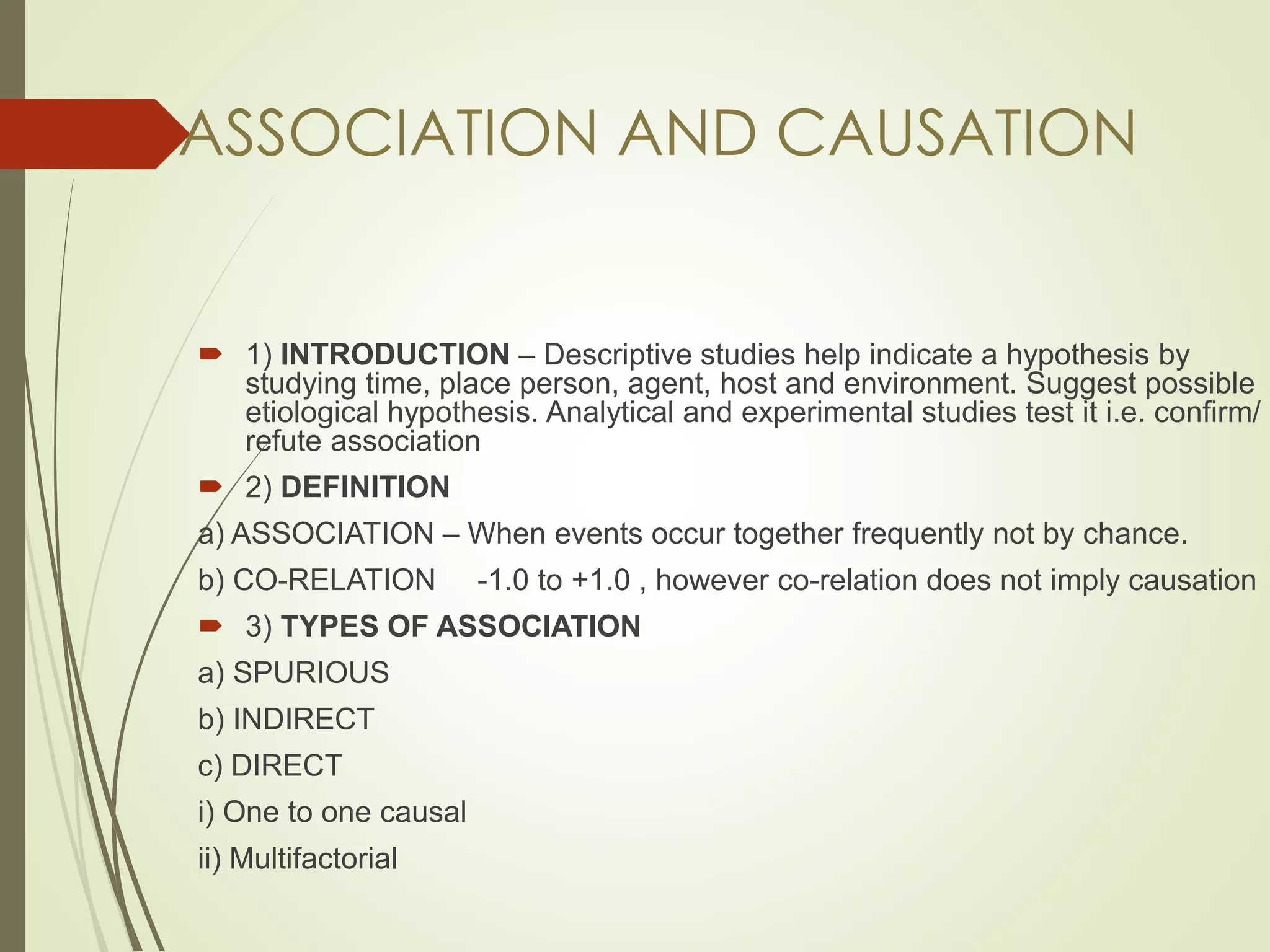
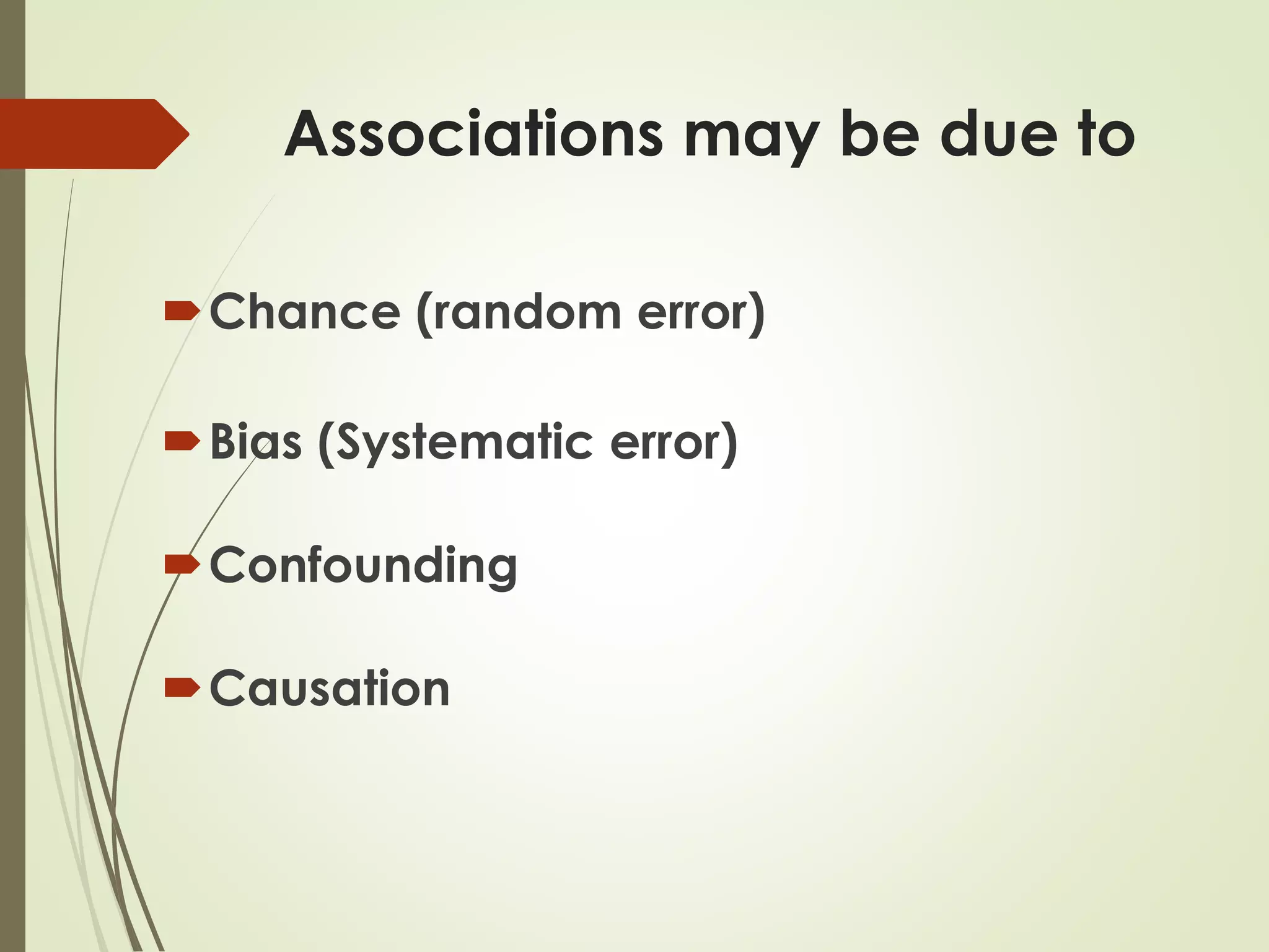
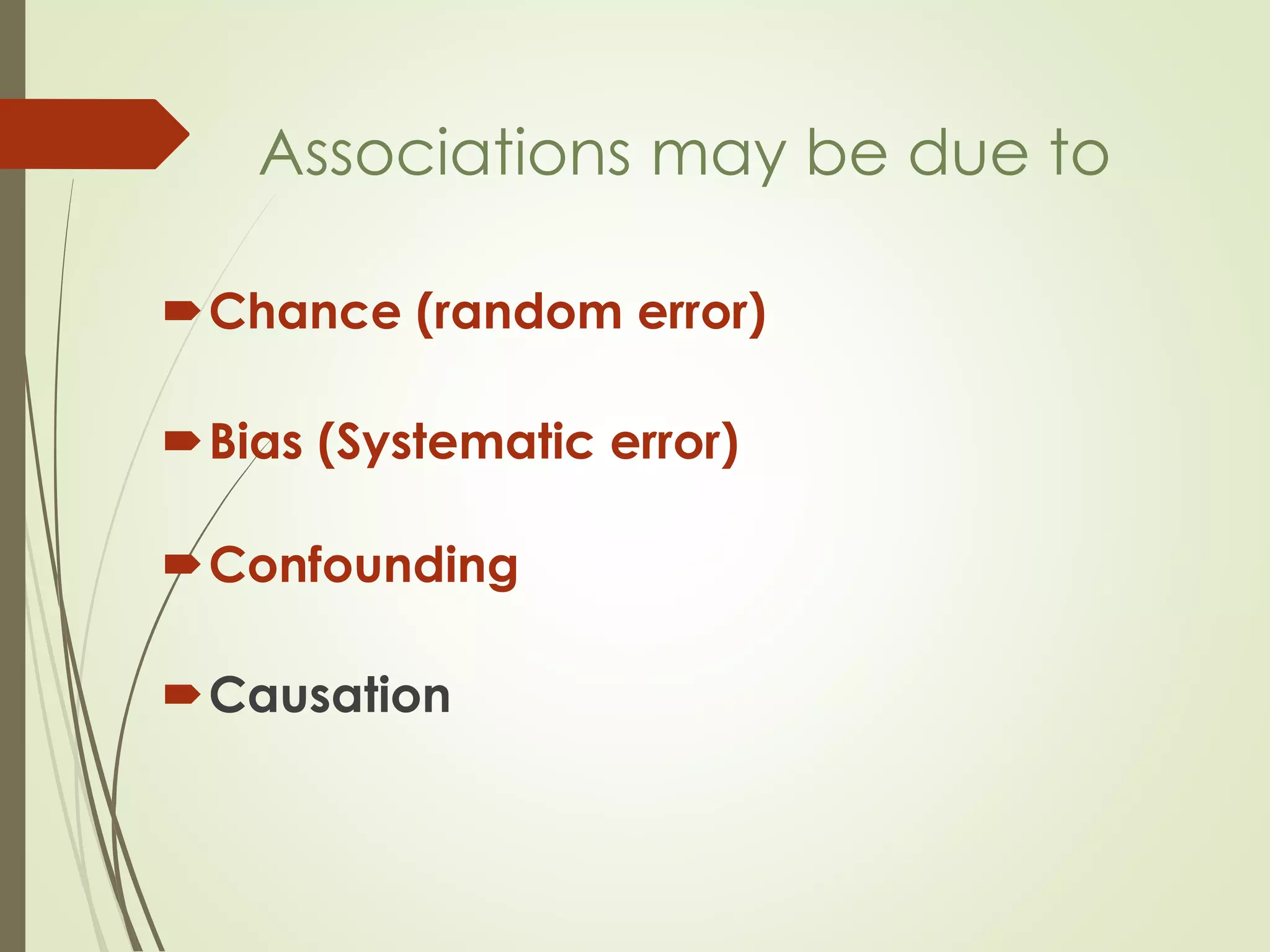
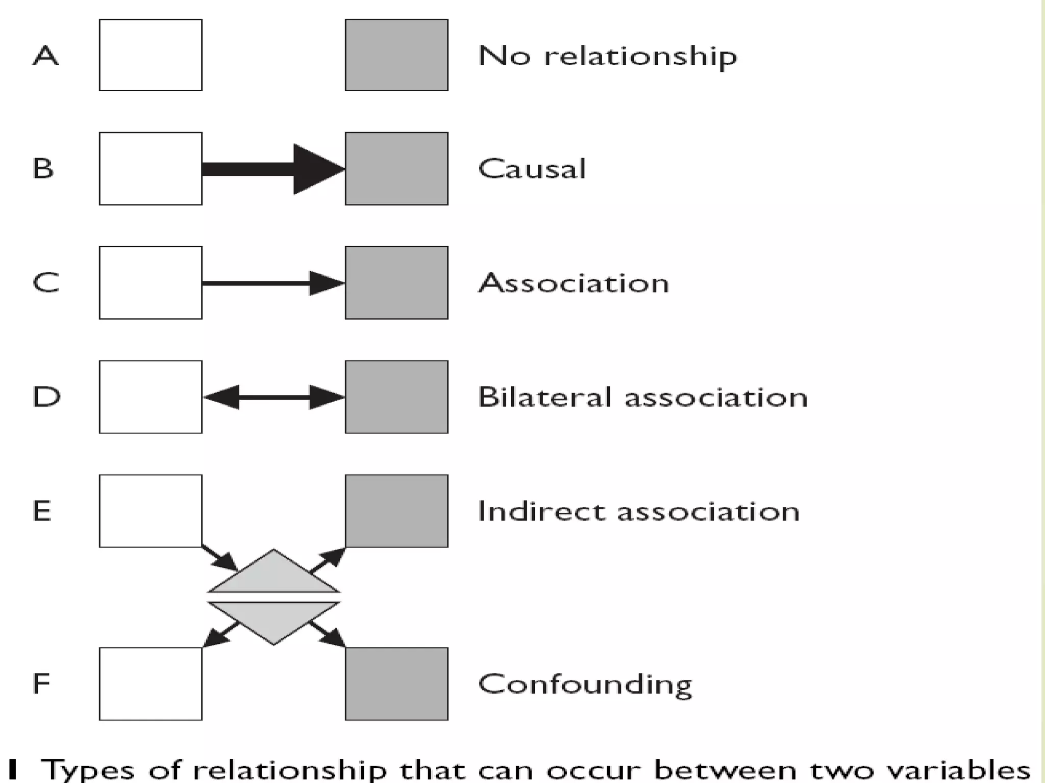
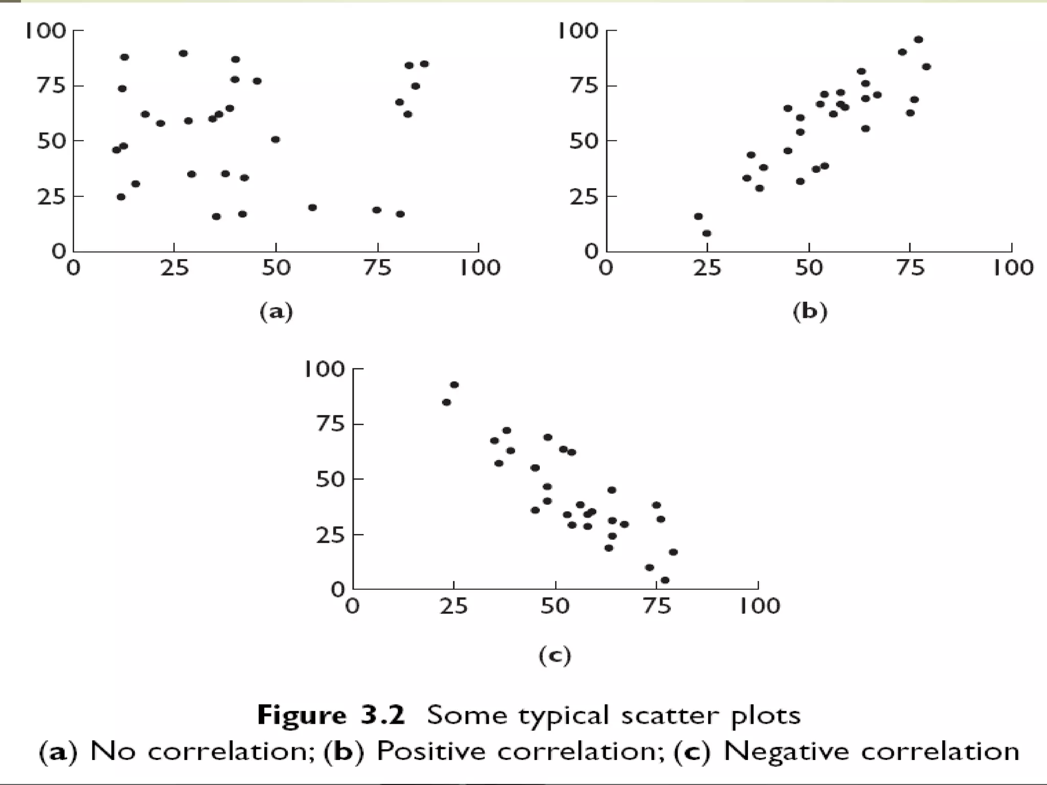
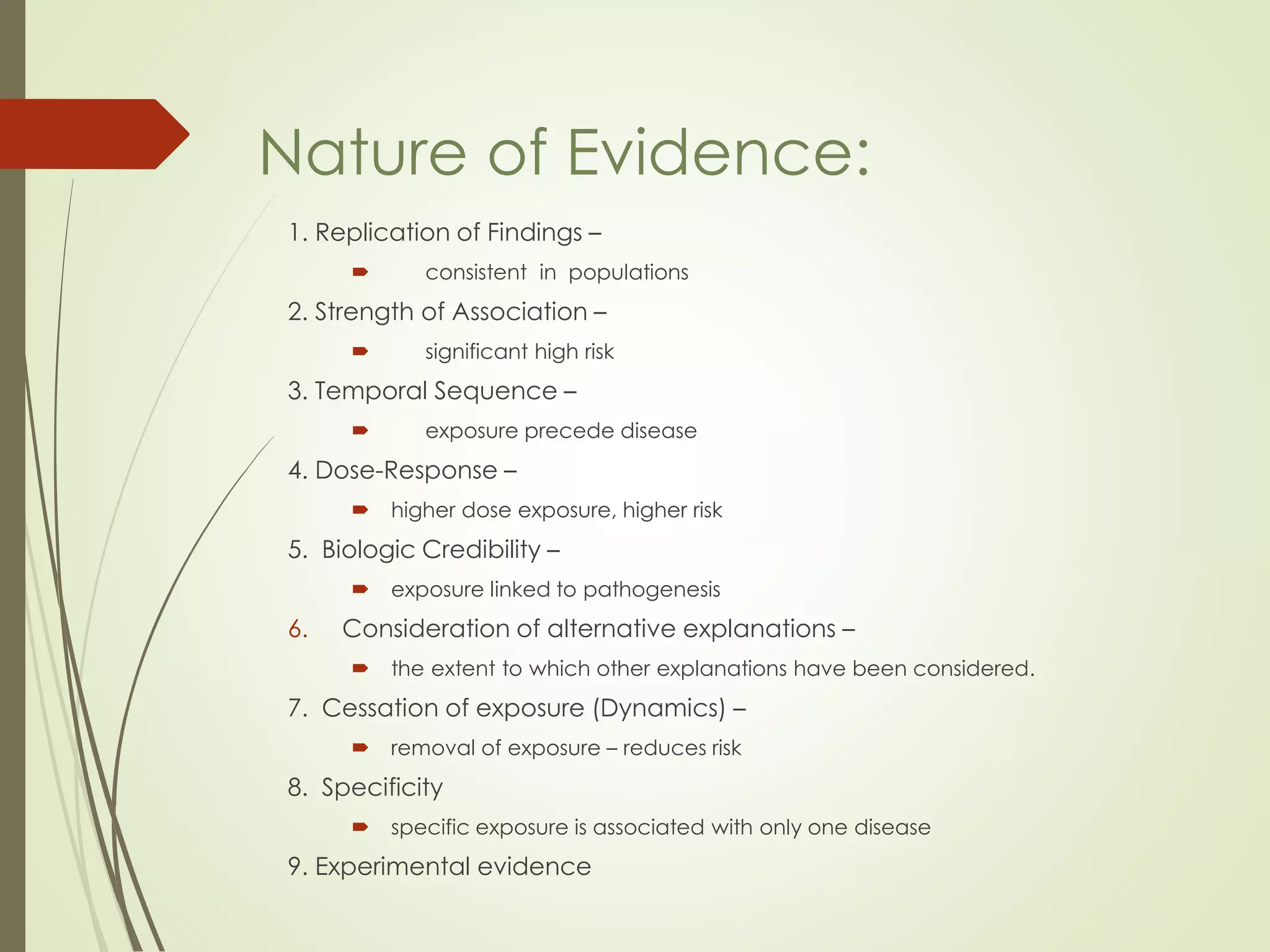
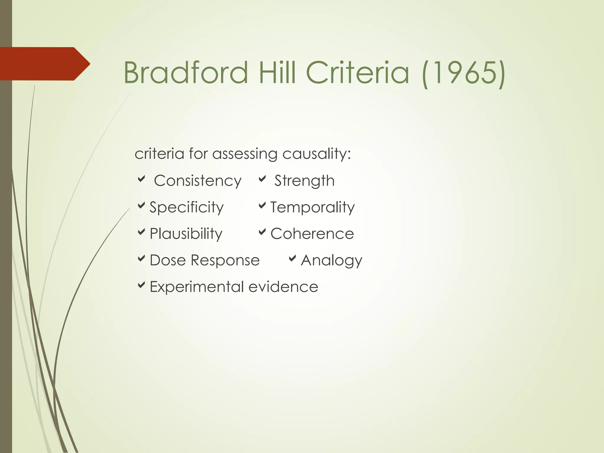
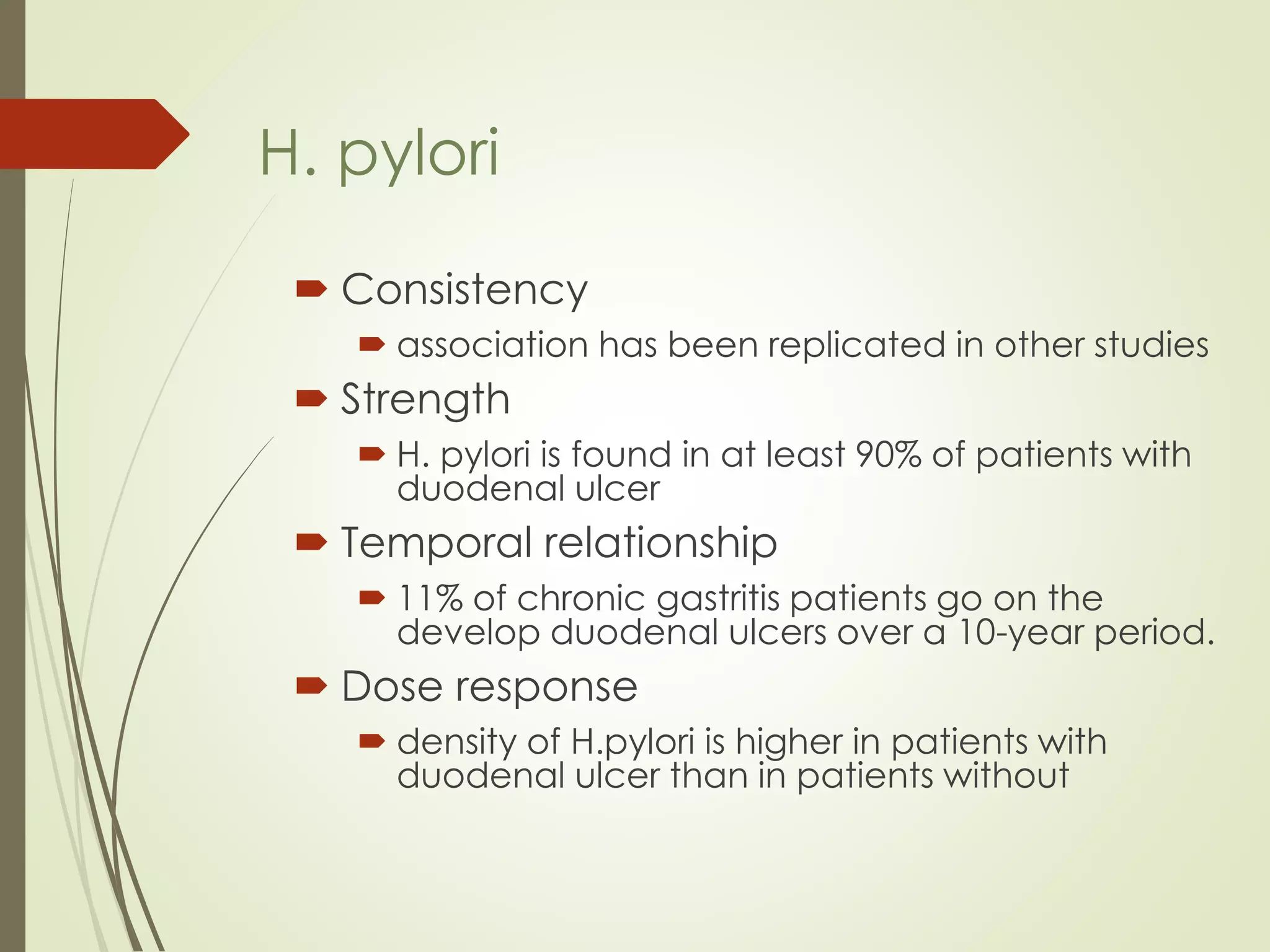
10-Interpretation& Causality by Mehdi Ehtesham

Interpretation& Causality
By: Mehdi Ehtesham
MPH/ Epidemiologist,
Avicenna Research Consulting
London, UK

ASSOCIATION AND CAUSATION
 1) INTRODUCTION – Descriptive studies help indicate a hypothesis by
studying time, place person, agent, host and environment. Suggest possible
etiological hypothesis. Analytical and experimental studies test it i.e. confirm/
refute association
 2) DEFINITION
a) ASSOCIATION – When events occur together frequently not by chance.
b) CO-RELATION -1.0 to +1.0 , however co-relation does not imply causation
 3) TYPES OF ASSOCIATION
a) SPURIOUS
b) INDIRECT
c) DIRECT
i) One to one causal
ii) Multifactorial

Associations may be due to
Chance (random error)
Bias (Systematic error)
Confounding
Causation

Dealing with chance error
 During design of study
 Sample size
 Power
 During analysis (Statistical measures of chance)
 Test of statistical significance (P value)
 Confidence intervals

Statistical measures of chance I
(Test of statistical significance)
Observed association
Association in Reality
Yes No
Yes
No
Type I
error
Type II
error

P-value
the probability the observed results
occurred by chance
the probability that an effect at least
as extreme as that observed could
have occurred by chance alone,
given there is truly no relationship
between exposure and disease (Ho)
statistically non-significant results are
not necessarily attributable to
chance due to small sample size

Statistical Power
 Power = 1 – type II error
 Power = 1 - ß

P value
Clinical Importance
VS
Statistical Significance

Statistical measures of chance II
(Confidence intervals)

Question?
 20 out of 100 participants: 20%
 What is the difference?

Answer: Confidence Interval
 Definition: A range of values for a variable of interest
constructed so that this range has a specified probability of
including the true value of the variable for the population
 Characteristics:
 a measure of the precision (stability) of an observed effect
 the range within which the true magnitude of effect lies with a
particular degree of certainty
 95% C.I. means that true estimate of effect (mean, risk, rate) lies
within 2 standard errors of the population mean 95 times out of
100
 Confidence intervals get smaller (i.e. more precise or more
certain) if the underlying data have less variation/scatter
 Confidence intervals get smaller if there are more people in your
sample

95% Confidence Interval (95%
CI)
95% CI: 12 to 28
95% CI: 16 to 24
95% CI: 19.2 to 20.8

Bias
 Any systematic error that results in an incorrect
estimate of the association between risk factors and
outcome

Types of Bias
Selection bias – identification of
individual subjects for inclusion in
study on the basis of either exposure
or disease status depends in some
way on the other axis of interest
Observation (information) bias –
results from systematic differences in
the way data on exposure or
outcome are obtained from the
various study groups

Selection Bias
 Self-selection bias
 Healthy (or diseased) people may seek out participation in
the study
 Referral bias
 Sicker patients are referred to major health centers
 Diagnostic bias
 Diagnosis of outcome associated with exposure
 Non-response bias
 Response, or lack of it, depends on exposure
 Differential loss to follow-up
 Exposed (or unexposed) group followed with different
intensity
 Berkson’s bias
 Hospitalization rates differ for by disease and
presence/absence of the exposure of interest

Information Bias
 Data collection bias
 Bias that results from abstracting charts, interviews
or surrogate interviews
 Recall bias
 Disease occurrence enhances recall about
potential exposures
 Surveillance or detection bias
 The exposure promoted more careful evaluation for
the outcome of interest
 Reporting bias
 Exposure may be under-reported because of
attitudes, perceptions, or beliefs

Bias results from systematic
flaws
 study design,
 data collection,
 analysis
 interpretation of results

Control of Bias
 Can only be prevented and controlled during the
design and conduct of a study:
 Careful planning of measurements
 Formal assessments of validity
 Regular calibration of instruments
 Training of data collection personnel

Confounding
 Confounding results when the effect of an exposure
on the disease (or outcome) is distorted because of
the association of exposure with other factor(s) that
influence the outcome under study.

Confounding
Coffee MI
Smoking,
Stress
Observed association, presumed causation
Observed association
True association

Properties of a confounder
A confounding factor must be a risk
factor for the disease.
 The confounding factor must be
associated with the exposure under
study in the source population.
The confounder cannot be an
intermediate step in the causal path
between the exposure and the
disease.

Control of Confounding
 During design of study
 Restriction
 Matching
 Randomization
 During analysis
 Stratified analysis
 Multivariate analysis

Coffee drinking
Myocardial Infarction
Yes No
Yes
36 24
No
24 36
OD= ?
OD = 36×36/24×24
OD= 2.25
Is there any confounding effect?

Stratification
Coffee
Drinking
Myocardial
Infarction
Yes No
Yes 2 6
No 18 34
Coffee
Drinking
Myocardial
Infarction
Yes No
Yes 34 18
No 6 2
Coffee
Drinking
Myocardial
Infarction
Yes No
Yes 36 24
No 24 36
Smokers
Non
Smokers

Coffee
Drinking
Myocardial
Infarction
Yes No
Yes 2 6
No 18 34
Coffee
Drinking
Myocardial
Infarction
Yes No
Yes 34 18
No 6 2
Smokers
Non Smokers
OD= ?
OD = 34×2/18×6
OD= 0.63
OD= ?
OD = 2×34/6×18
OD= 0.63
Stratification

Crude OR = 2.25
Common OR = 0.63
So
There is confounding effect.
Crude and Common OR

Chance (random error)
Bias (Systematic error)
Confounding
Causation
Associations may be due to

The numerical value ascribed to these relationships is the correlation coefficient, its
value ranging between +1 (a perfect positive correlation) and −1 (a perfect negative
correlation).
Pearson’s and Spearman’s are the two best-known correlation coefficients. Of the
two, Pearson’s product–moment correlation coefficient is the most widely used, to
the extent that it has now become the default. It must nevertheless be used with
care as it is sensitive to deviations from normality, as might be the case if there were
a number of outliers.
With the correlation coefficient, the +/− sign indicates the direction of the
association, a positive correlation meaning that high values of one variable are
associated with high values of the other. A positive correlation exists between height
and weight, for example.
Conversely, when high values of one variable usually mean low values of the other
(as is the case in the relationship between obesity and physical activity), the
correlation will be negative.
Correlation coefficients

In addition to the problems related to normally distributed data, correlation
coefficients can be misused in other ways. Detailed below are some of the most
common ways in which such misuse tends to occur:
• When variables are repeatedly measured over a period of time, time trends can
lead to spurious relationships between the variables
• Violating the assumption of random samples can lead to the calculation of invalid
correlation coefficients
• Correlating the difference between two measurements to one of them leads to
error. This typically occurs in the context of attempting to correlate pre-test values to
the difference between pre-test and post-test scores. Since pre-test values figure in
both variables, a correlation is only to be expected
• Correlation coefficients are often reported as a measure of agreement between
methods of measurement whereas they are in reality only a measure of association.
For example, if one variable was always approximately twice the value of the other,
correlation would be high but agreement would be low.

 The general QUESTION:Is there a cause and effect
relationship between the presence of factor X and the
development of disease Y?
 One way of determining causation is personal
experience by directly observing a sequence of
events.
DETERMINATION OF CAUSATION

 Long latency period between exposure and disease
 Common exposure to the risk factor
 Small risk from common or uncommon exposure
 Rare disease
 Common disease
 Multiple causes of disease
Personal Experience / Insufficient

The answer is made by
inference and relies on a
summary of all valid
evidence.
Scientific Evidences

1. Replication of Findings –
 consistent in populations
2. Strength of Association –
 significant high risk
3. Temporal Sequence –
 exposure precede disease
4. Dose-Response –
 higher dose exposure, higher risk
5. Biologic Credibility –
 exposure linked to pathogenesis
6. Consideration of alternative explanations –
 the extent to which other explanations have been considered.
7. Cessation of exposure (Dynamics) –
 removal of exposure – reduces risk
8. Specificity
 specific exposure is associated with only one disease
9. Experimental evidence
Nature of Evidence:

criteria for assessing causality:
 Consistency  Strength
Specificity Temporality
Plausibility Coherence
Dose Response Analogy
Experimental evidence
Bradford Hill Criteria (1965)

 Hill stated
 None of my criteria can bring indisputable evidence for
or against the cause-and-effect hypothesis
 None can be required as sufficient alone
Bradford Hill Criteria

 Consistency
 association has been replicated in other studies
 Strength
 H. pylori is found in at least 90% of patients with
duodenal ulcer
 Temporal relationship
 11% of chronic gastritis patients go on the
develop duodenal ulcers over a 10-year period.
 Dose response
 density of H.pylori is higher in patients with
duodenal ulcer than in patients without
H. pylori

 Biologic plausibility
 originally – no biologic plausibility
 then H. pylori binding sites were found
 know H. pylori induces inflammation
 Cessation
 Eradication of H Pylori heals duodenal ulcers
H. pylori

1. Strength of Association:
 The relative risks for the association of smoking and lung
cancer are very high
2. Biologic Credibility:
 The burning of tobacco produces carcinogenic compounds
which are inhaled and come into contact with pulmonary
tissue.
SMOKING AND LUNG CANCER

3. Replication of findings:
 The association of cigarette smoke and lung cancer is found
in both sexes in all races, in all socioeconomic classes, etc.
4. Temporal Sequence:
 Cohort studies clearly demonstrate that smoking precedes
lung cancer and that lung cancer does not cause an
individual to become a cigarette smoker.

5. Dose-Response:
 The more cigarette smoke an individual inhales, over a
life-time, the greater the risk of developing lung cancer.
6. Dynamics (cessation of exposure):
 Reduction in cigarette smoking reduces the risk of
developing lung cancer.

 Smoking is cited as a cause of lung cancer, however. . .
 . . . smoking is not necessary (is not a prerequisite) to get lung cancer.
Some people get lung cancer who have never smoked.
 . . . smoking alone does not cause lung cancer. Some smokers never get
lung cancer.
 Smoking is a member of a set of factors (i.e., web of causation)
which cause lung cancer.
 The identity of all the other factors in the set are unknown. (One factor in
the web of causation is probably genetic susceptibility.)

D
E A
B
C F
B
AH
G
F
C
AJ
I
“A” is necessary – since it appears in each sufficient
causal complex
“A” is not sufficient –
Disease Not Present Disease Present Disease Present
necessary / sufficient

 necessary and sufficient
 the factor always causes disease and disease is never present
without the factor
 most infectious diseases
 necessary but not sufficient
 multiple factors are required
 cancer
 sufficient but not necessary
 many factors may cause same disease
 leukemia
 neither sufficient nor necessary
 multiple cause

 Few causes are necessary and sufficient
 High cholesterol is neither necessary nor sufficient for CVD
because many individuals who develop CVD do not
have high serum cholesterol levels

10-Interpretation& Causality by Mehdi Ehtesham

More Related Content

What's hot

Viewers also liked

Similar to 10-Interpretation& Causality by Mehdi Ehtesham

10-Interpretation& Causality by Mehdi Ehtesham