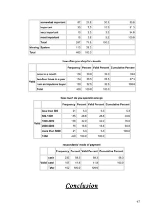
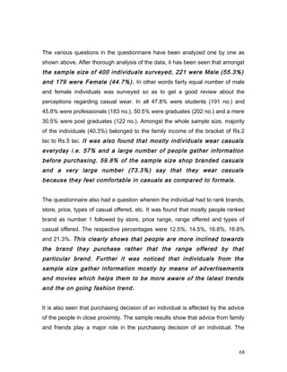
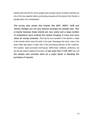
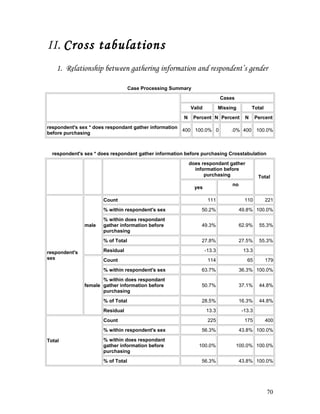
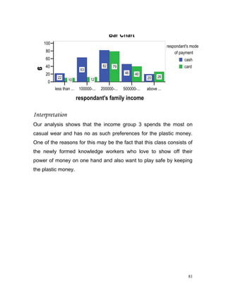
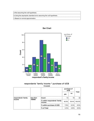
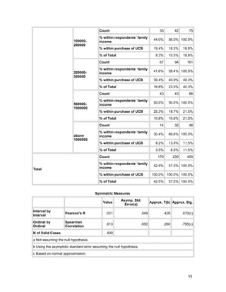
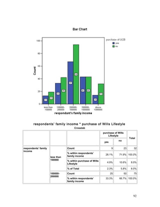
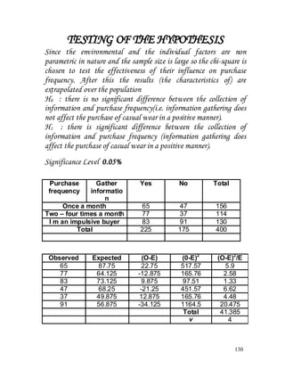
NewBase 19 April 2024 Energy News issue - 1717 by Khaled Al Awadi.pdf
casual wear
1. MARKET RESEARCH
Study of Consumer Decision Making
Process for Casual Wear
Group Members:
Aman Jain – A02
Jaya Kumari – A19
2. Sachin Sehgal – A35
AMITY BUSINESS SCHOOL
NOIDA
Certificate of Appreciation
This is to certify that Aman Jain, Jaya Kumari
and Sachin Sehgal carried the project titled
“Study of Consumer Decision Making
Process for Casual Wear” under my guidance
and supervision as a part of their academic
curriculum towards the partial fulfillment of the
PGDM program.
I wish them all a bright future and good luck.
2
4. Acknowledgement
This research project would have been a babbling effort and a
bumpy ride if our Project Guide Dr. S.K. Laroiya would
not have been shining like a beacon throughout the whole
journey of this mammoth effort. We as a team would like to
sincerely thank him for his support and guidance without
which it many a times seemed impossible to bring the project
to its present form.
We are obliged towards all the respondents for
providing us with the information we required. We thank
them all for their giving their valuable time to us.
In the end we would like to thank all those who have
helped us while completing this research project and who
have become an integral part of this project. We dedicate this
project to all of these people.
The obliged team:
Aman Jain - A02
Jaya Kumari - A19
Sachin Sehgal - A35
4
5. Research Objectives
After a brainstorming session with the group members and the
project guide, the following are the objectives of the project:
• To study the consumer decision making process for casual
wears in the age group of 15-25 years in Delhi and NCR
region.
• To study the various factors influencing purchase decisions
for the casual wear.
5
6. Introduction
Casual wear is considered to be the inevitable part of our lives. These
are clothes which help us feel comfortable, in sync with the times and
above all help us to feel at home. The biggest advantage of wearing a
casual is the psychological effect that erases off the strict rules and
discipline of the formal wear and its boundaries. Be it Indian, western
or indo-western casual wears come in many shapes, sizes, designs
and with loads of fun. This perhaps is the reason why the students on
the verge of going to college, we interviewed seemed so excited
about the idea of going to college just because they will be able to
wear whatever they want! And for that matter this means casual
wear. Casual wear today perhaps are synonymous with unlimited fun,
frolics and hungamas.
Casual wear forms an integral part of our lives. There is bigger
picture showing the serious business behind the casual wears. The
casual wear business in India is more than $5000 million per year.
This is the data for the organized branded casual wear and does not
include the blooming businesses of the non-branded casual wear in
the markets like Sarojini Nagar, Lajpat Nagar, Chandini Chowk etc.
as per a rough estimate only Chandini Chowk makes a whopping
business of few hundred crores daily by selling suits only, a type of
Indian casual wear for ladies.
Branded ready-to-wear (RTW) is the latest craze not just among
consumers, but textiles and fabrics majors. Despite severe
competition from the highly fragmented industry — whose size is
6
7. anywhere between Rs 15,000 crore to Rs 20,000 crore — the annual
growth rate of over 20 per cent with high visibility and impressive
margins is what has attracted textiles majors like Century Textiles,
Indian Rayon, Raymonds, Bombay Dyeing among others to this
industry.
Interestingly, cashing in on the popular men’s RTW, it is the RTW for
women which are the latest trend that’s being used to expand the
market further. And the lead in ladies RTW has been taken by Indian
Rayon which recently launched its maiden ‘Allen Solly — Ladies
Wear’ range of products. This important shift in marketing strategy
would soon be followed even by Century Textiles. Raymonds last
year already launched the pret line for women under the label of BE
which is available in upmarkets of both New Delhi and Mumbai.
The whole growth strategy is to acquire and introduce newer ranges
like ladies RTW, casual wear, sports wear etc.
The textile majors used the acquisition route to enter the apparel
business. Raymonds recently acquired ColorPlus for entering the
casual wear thereby adding to its own existing formal wear under the
names of Parx, Raymonds, and Park Avenue. Indian Rayon used this
strategy by taking over the garments division of Madura Coates thus
entering the apparel business with the prestigious Allen Solly, Van
Heusen, Louis Phillpe and Peter England range of formal mens wear,
while Bombay Dyeing too took over Proline to enter the sports wear
while adding to its existing formal mens wear under Vivaldi range.
7
8. Analysts said this trend would continue in future with more such
acquisitions of successful brands (in the unorganised sector) being
taken over by successful players. With such a strategy, the company
gets a ready market captured by the existing brand while also helping
the company to avoid critical brand-building activities, they said.
Further, analysts attributed this trend as a logical move towards
building the value chain to their own textiles manufacturing. This burst
of RTW is also due to the growing potential that these companies see
in the growing working population women besides men, leading to
rising income levels, due to more disposable income.
Raymonds president Nabankur Gupta said, “Raymonds wants to
consolidate and expand its existing range of apparel brands and we
are open to the idea of takeovers and acquisition in this sphere.”
Besides, the textile companies are leveraging the existing distribution
and retailing network of the fabrics market available to them, this will
help them in introducing products. According to Mr Gupta,
“Raymonds boasts of an extensive retail network of over 13,000
retailers in over 400 town and cities, in India and abroad.”
However, the smaller players do not feel the threat of cannibalisation
yet they feel that target consumer for them is different. Cambridge
Enterprises partner Narendra Bhatia said, “The Cambridge brand of
meanswear is positioned for mass market and companies like
Raymonds are targeting the middle and the upper class customers.”
8
9. Indian Rayon director Vikram Rao said, “We are targeting the middle
and higher end of the market only by finely differentiating the product
price. However, we are not targeting the mass market since our
economics is not met by pricing the products for that segment.
Indian Rayon’s strategy, said Mr Rao, is to introduce whole range of
not just RTW but also accessories, leatherwear and other related
products.
Analysts said these and other players in the segment would try and
diversify in various segments of apparels so that they can tap all
segments of the market for overall growth.
However, as compared to the global RTW market, estimated at
around $183 billion India’s RTW is just in a nascent stage where
players hope to expand faster than their competitors.
Besides, players in the domestic apparel industry felt that there is no
fear of foreign competition in their segment as costs of introducing
apparel in India will be very expensive for these players. Mr Vikram
Rao said, “We expect foreign players to come in maybe in 3-5 years
but they are most likely to adopt the retail outlet to offer their
products.”
This trend will be on the increase as the companies are looking at
growth potential from each and every segment of apparel. However,
the companies have to face tremendous competition from the
unorganised sector as well as smaller players as well.
9
10. Thus, to differentiate from the clutter of the mass market segment the
companies have also planned a strategy of standardising the
products.
For this, the companies are introducing standard sizes to body
shapes like the newly introduced Allen Solly range for women comes
in comfort, regular, straight and trim fits. The companies are
upgrading the consumers by bringing in this segment said analysts.
As compared to the global industry which is nearly of $183 billion, the
domestic readymade industry is still in a nascent stage. The structure
of the readymade industry in India is complex as much as it is
diverse. It is highly fragmented and a large part of it is unorganised.
However, trend forecasters said that these companies would get into
the entire value chain by entering into kids wear, sports wear etc. The
companies, which do not manufacture fabrics for sportswear and kids
wear, may start doing so and enter this segment. Also, the
companies would keep introducing newer varieties, styles, and
collection in different seasons and for different occasion to keep the
consumers attracted and get a bigger slice of the pie.
Pantaloon Fashions managing director Kishore Biyani said, “The
trend is shifting more from tailored clothes to readymade garments,
due to easy availability and affordable prices.”
The companies are offering clothes at a very affordable price,
besides, the convenience of picking clothes off the rack gives the
10
11. customer a certain surety of look and the finish, which is missing in
the tailormade clothes.”
The pricing is done keeping in mind the perceptible value of the
product, the clothes more often than not are priced at around the
tailored wear’, added Mr Biyani.
A number of brands like ColorPlus, Provogue, Tamarind have
established a foothold in the ready-to-wear market. The branded
apparel market in India is dotted with numerous such brands
marketed by umpteen players. What separates one from the other is
the USP that each one attempts to create to attract customers to their
stores. Color of the garment is a key differentiator, while design,
fabric and finish are the others.
The research basis of this report is Casual wear. Casual wear is
defined as the informal attire which people wear to workplaces on
weekends, students wear other than school, etc. all in all on one hand
the attire in which people feel free and on the other the attire which
can not be worn for a formal meeting, get together, dinner or any
such occasion.
We have divided the range of casual wear into the following classes:
- Jeans
- Skirts
- Capris
- Jackets
11
12. - T-Shirts
- Sandoz
- Suit (for girls)
- Shorts
- Three-fourths
- Bermudas
- Knickers
- Sports wear
- Cargos
- Chinos
- Six pockets
- Parallel
The report studies in the succeeding pages studies what exactly
does a customer feels while going to purchase a casual wear,
why does customer buys, does he(she) only for him(her)self, does
he gather information before purchasing a casual wear and if yes
why so and so many similar things. All this has helped us
understand the consumer decision making process for a casual
starting from the need recognition till the disposing off the product.
This report also studies the influence of the environmental and
personal factors while purchasing the product.
12
13. The Current Market Scenario
The current market scenario of the casual wear portrays a picture of
highly competitive, fast moving market comprising of highly
demanding, distinguishing and even highly discriminating customers.
The fast moving customers who in turn are influenced by even fater
moving fashion trends all over the world characterize the market. The
accessibility of information, increasing purchasing power, changing
lifestyles and social setups and most importantly the changing values
are the drivers of this casual wear market.
This market many a times seems to be highly confused,
disintegrated and unorganized and suddenly it seems to be a highly
profitable place for the companies and fashion houses all over the
world and as a result reputed fashion houses like Chanel, Versache,
Louis Vouitton, Christian Dior etc. are a part of the band wagon
joining the great India shining ride. And many more brands of such
repute are preparing to join the same very soon.
Coming back to India the sudden surge in the fashion industry
with two big events lined (after the infamous break up of lakme with
India fashion week) has definitely helped the designers to reap the
opportunities lined up. Bollywood has also emerged as a big platform
for these designers to showcase their latest collection to the masses
and reach them in no times. The recent waves of fashion trends can
be quoted as examples hit movies like Kabhi Khushi Kabhi Gam, Kal
Ho Na Ho, Lakshya, Salam Namaste etc have set up fashion trends
and as a result the markets are flooded with skirts, from boot cuts to
13
14. straight fit jeans, head gears, suits in latest indo western styles and
so on. The movies in India have also motivated some big fashion
houses like DKNY(with Kabhi Khushi Kabhi Gam) to enter into Indian
markets.
Despite all the rosy picture portrayed so far the reality is hard hitting.
The market in reality is brutal and un forgiving. It’s a place where
winning is the sole criteria of survival that too in a market which
shows great colors in terms of big and improving purchasing power
and changing lifestyles but all this statistics are limited to the realms
of the big metros. The wave of branded casual wear and standard
has not yet reached the outskirts of India. Recently released Forbes
World’s richest shows that out of the 102 new entrants of the club
“riche rich” 11 are Indians that means 1 out of every 10 new
billionaires joining the Forbes list is an Indian. This can naturally be
the dream market to launch the product with a bang. However this
dream is turning sour for many of the foreign brands United Colors Of
Benetton, Lacoste etc can be cited as example. United Colors of
Benetton has already packed up its operations in India. The market is
not as easy to conquer as it seems to be. Price is a criteria but not
the sole, size does matter, stores also, then relationships with the
“purane wale bhaiyya” comes in picture, and above all the class,
income levels and perceptions. The recent studies show that in India
the emerging middle class is the most spendthrift of all earning
between Rs. 200000-Rs.500000 per annum, families where both the
parents are working with one or two kids to look after. This is the
14
15. class that spends the most expecting to be counted in the upper
classes. However, the most heart breaking class is the class earning
between Rs. 500000-Rs.1000000 per annum and above it. This is the
class that spends the less but is instrumental in bringing the world
class labels to the country.
Textile : Overview
Textiles Industry: Market Rs. 207,895 crores* (US$ 48346 million)
Process Products Machines Mills/ Units
Spinning
(Rs. 34700
crs.
US $ 8070
mln)
Yarn Spindles,
Rotors
Spinning Mills
Composite Mills
EOUs
Weaving
(Rs. 148960
crs.
Fabric Looms Power Looms
Hand Looms
Composite Mills
15
16. US $ 34640
mln)
Finishing
(Rs. 24235 cr.
US $ 5636
mln)
Garments Processing and
Stitching
machines
EOUs & SSIs
* Estimated 2004-05
• Largest organised sector industry in India - has a 20%
weightage in Index of Industrial Production
• Largest export earner; second largest employer - > 20 million
people.
• Cotton dominant fibre; polyester/ cotton blended yarn and
fabrics catching up
• Ready made garments (RMG) - a part of the finished textiles
process
RMG Industry: An Overview
• Industry has grown rapidly since early ‘90s
• Value-adds to fabrics around 40%, through design and
marketing
• Makes up 15% of country’s export earnings - single largest net
forex earner
16
17. • Concentrated in unorganised sector - employs around 2.5
million workers
Category Range Some Brands
Formal Wear Suits, Trousers, Shirts,
Jackets Blazers,
Neckties…...
Allen Solly, Arrow, Cambridge,
Colour Plus, Louis Philippe, Peter
England, Park Avenue, Reid &
Taylor, San Frisco, Van Heusen
Casual Wear Shirts, Trousers, Jeans,
Tee Shirts Shorts,
Lee, Flying Machines, Parx,
Weekender, Wear-house,
Benetton
Kids wear Shirts, Shorts, Frocks,
Skirts,
Jeans….
Lee, Ruf ‘n’ Tuf, Wear-house,
Weekender
Ladies Wear Skirts, Tops, Salwar
Kameez ,
Sarees
No national brands
Under
garments
Knitwear
Vests, Briefs, T-Shirts,
etc.
Byford, Crocodile, Jockey, Park
Avenue, Tantex, VIP, Jockey,.
RMG Industry : Market
17
18. • Annual output 1998-
99: Rs. 24,235 crs
(US $ 5636 mln), at
an estimated 10980
million pieces
• Cotton garments had
a growth around 2.5%
while blended
garments had a higher
rate around 9%
Raw Material
• Key input : Cotton - available abundantly in the country (80% of
market is for cotton garments).
• High - quality fabrics also imported under advance licencing
scheme.
Industry Structure
• Highly fragmented; Market dominated by unorganised sector
(>60%) over 50,000 units in operation : each has typically 15-20
machines
• Smaller players also active in local and overseas markets
• Larger players positioned in branded segments - Arvind Mills,
Madura Coats, J K Synthetics.
18
19. • Concentration of units in Tirupur (Tamil Nadu) - major centre for
cotton and knitted garments,(exports and domestic); also at
Bangalore, Chennai Mumbai and N Delhi
RMG Industry : Exports
RMG an export oriented industry
o These exports are either done by units on their own or
through export houses
o India’s RMG exports are around Rs. 22650 crs US $ 5267
mln), as against the global demand of over Rs. 688,000 crs. (US $
160,000 millions)In the world market, India’s share (3%);China (15%),
Hongkong (13%) and Italy (8%); other competitors - Pakistan,
Indonesia, Thailand, Egypt
o Labour cost in India is very cheap; Per hour rates :India :
US $ 0.72; Hong Kong - US$ 3.05, Japan - US$ 13.96, Singapore -
US$ 2.83
o Focus on exports aided by governmental policies;the
latest textile policy announced in Nov ‘99 encourages units to enter
non-quota markets.
Indian exports are mainly to quota countries (> 60%) - USA (> 20%) ,
Germany, UK, France, Canada Non-Quota markets : CIS, Gulf,
Japan,Switzerland and Australia
19
20. State-wise share of exports
Readymade Garments : WTO Implications
• Upto 1995, textile trade regulated by Multi Fibre Agreement
(MFA) - enabled importing countries(mainly Western) to impose
quota restrictions on exports from developing countries
• Quotas imposed on selective basis - India and Pakistan
clubbed together with lower quota, Srilanka marginally higher
quota, Bangladesh with no quota and so on
• With the formation of World Trade (WTO) in January 1995,
MFA replaced by Agreement on Textiles and clothing (ATC);
MFA to be phased out over a 10-year period from 1995
• Scope for increased market access during the transition period
of 10 - years for products under quota system
• Market size of quota-imposing countries large - exports could
become more competitive.
• Indian exporters stand to gain with the opening up of markets
hitherto restricted.
20
21. Readymade Garments : Market Segmentation
Players Major Brands
Arvind Mills
Unit: Bangalore
Casuals: Lee, Flying Machine,
Newport, Ruf 'n' Tuf, Ruggers.Shirts:
Arrow, Excalibur
Madura Coats,
Bangalore
Shirts: Allen Solly, Louis Philippe, Peter
England, Van Heusen; Trousers: San
Frisco;
T- Shirts & Socks - Byford
J K Synthetics Park Avenue range of shirts, Trousers,
T- Shirts, Under garments, Belts, etc.
Parx range of casuals
21
22. Readymade Garments : Market Characteristics
Key Success Factors
• Branding & sub branding
• Offering variety : current trends and patterns
• Coping with change in fashion quickly
• Quality standards - in material, stitching, cuts
• Moving up the value-chain - ensuring better returns
• Export market - Sticking to delivery schedules, honouring
quality and quantity commitments, ability to interpret fashion
changes
Market Characteristics
• Highly dynamic - designs changing frequently
• Brand consciousness catching on-focus on quality, finish; price
secondary a factor.
• Increasing competition in the branded segment.
• Some major players target different customer segments within
the same product line with different product offerings. For e.g.,
Arvind Mills has positioned its denims “Lee” at Premium
casuals, “Flying Machine” at upper -end casuals and “Newport”
as a value-for-money brand
22
23. • Active Trade Channel - 4 types of channels used : Franchises
(Benetton)/ Exclusive stores (Arvind Mills); Outright Sales to
retailers (Louis Philippe); Company-owned stores (Colourplus);
Normal 3 - tier chain through stockists, distributors, retailers
(Louis Philippe). Some players opt for multiple channels also
(Louis Phillip, Colourplus)
• Significant expenditure on marketing / brand building only for
branded segment
• Local manufacturers have tied-up with foreign brands (Arvind
Mills sells denims under ‘Lee’ label and “Arrow” shirts for Clue
Peabody & Co., US; DCM supplies under ‘Benetton’)
23
24. Readymade Garments : Future
Business Concerns
• In garment exports, lower prices realisation due to intense
competition - Pakistan a major force, has similar competitive
edge in cost structure
• Environmental issues : Ban on certain dyes and fabrics such as
rayon and insistence on usage of vegetable dyes have
impacted exports
• Raw material prices: Fluctuation in cotton prices (a commodity
product) has affected cost structures
Demand Drivers
• Rise in disposable income - burgeoning of middle class
• Fashion consciousness; etiquette, aesthetic appeal
• Convenience - purchase : available off the shelf
• Influence of western styles - media driven
• Export markets : Western countries looking to developing
countries to source cheaper products
Future
• The future for blended garments appear to be bright at around
9% annually.Cotton garments growth to stagnate. WTO
implications could positively impact industry in the long run
24
25. • Brand buy-outs - entry route for new and consolidation for
existing players
Summing up An export-oriented sector-prospects for exports
improving, domestic market slowly opening up.
25
26. Previous Studies On The Topic
This is the study done by KSA Technopak for the branded
and non branded wear. Some facts of the study are as
following:
• The top 40 cities of India account for almost 50% of Sec A&B
population
• Sec A&B contribute almost 98% to the branded segment
• The largest segment for clothing is the 16-35 age group (brand
name and quality are top priority)
• Branded segment is growing at 18-25% annually from 1998
onwards (the industry growth rate is only 5%)
• Branded wear accounts for more than 21% of the apparel
industry (around Rs 9,000 crore
-KSA Technopak
Our analysis of these figures:
Now, for what these figures mean. Simply that the Indian consumer
is showing an increasing fascination for branded wear. The reasons
are clear - one, the increased disposable income of Indian
households and two, the fast paced changes in the ready-to-wear
industry. Today's customers are fussier than ever before - they are
more aware of current trends, are totally in sync with the latest in
fashion and demand the best products as well as service at an
26
27. affordable price. And manufacturers and retailers are going all out to
keep them happy. Definitely, the ready-to-wear business is in vogue.
From 'mom-and-pop' shops to organised retail, from unbranded
merchandise to labels, from off-the-street quality to value for money,
the ready-to-wear sector is witnessing an upheaval. At the forefront of
all these changes are the highly versatile small brands. With big
brands from textile companies growing weary in adapting to the fast-
paced changing scenario in the ready-to-wear industry, it's the small
brands, including private labels that are completely transforming the
way men, women and children dress.
A whole bunch of players have plunged into this branded ready-to-
wear business. Easy to see why. According to current KSA
Technopak reports, the branded ready-to-wear segment contributes
only 21% to the apparel sector. And the present total market size of
the ready-to-wear segment is pegged at around Rs 40,000 - 45,000
crore.
That's lucrative indeed and there still is a lot of space for all to grow
and grow big. And once the supply chain constraints have been
eased, real estate markets made more organised and tax structure
rationalised, this sector will become quite irresistible. Says Arvind
Singhal, MD, KSA Technopak, "Ready-to-wear segment will be the
key driver in the textile industry in the next five years."
27
28. Research Design
The research design is the most important step in producing the
results in the form of usable conclusions. A research design is the
detailed blueprint used to guide a research study towards its
objective. The process of designing this research project has involved
various interrelated and interdependent steps. The choice of
information type, its gathering, analysis and interpretation of the
results were determined on the basis of this research design.
Phase 1 Preliminary Planning Stage
The research in question is basically a mix of the three types of
research starting with the exploratory research to define the problem
(objectives and premises) , then moving to the descriptive research
where the sample characteristics were explore and defined finally
moving to the most important type of the research design that is to
the casual research where the cause and effect relationship between
the various variables we found important during the first two phases
of the research process.
Step 1.Type Of Research.-Exploratory
In the first phase the following research framework was designed
after long brainstorming sessions within the group, with the project
guide and holding discussions with the potential respondents.
28
29. In the disruptive, discontinuous markets of contemporary and future
businesses environments, a “roadmap” of how consumers make
purchase decision is much more reliable than a set of “directions”.
The consumer decision process (CDP) model, a simplified version of
which is shown in the succeeding figure.
29
31. It represents a roadmap of consumers’ minds that marketers and
managers can use to help guide product mix, communication and
sales strategies. The model captures the activities that occur when
decisions are made in a schematic format and shows how different
internal and external forces interact and affect how consumers think,
evaluate and act.
As the model shows, consumers typically go through seven major
stages when making decisions: need recognition, search for
information, pre-purchase evaluation, purchase, consumption, post-
consumption evaluation and divestment. Though marketing textbooks
and consumer researchers sometimes employ slightly different
terminology for each of these seven stages and how various factors
influence each stage of consumers’ decisions. By understanding the
stages in the consumer decision-making roadmap, marketers can
discover why people are or are not buying products and what to do to
get them to buy more or from a specific supplier.
Stage 1 (Need Recognition):
31
32. The starting point of any purchase decision is a customer need. Need
recognition occurs when an individual senses a difference between what he or
she perceives to be the ideal versus the actual state of affairs. Consumers buy
things when they believe a product’s ability to solve a problem is worth more than
the cost of buying it, thereby, making recognition of an unmet need in the first
step. In addition to needs, consumers also have desires. While marketers strive
hard to fulfill desires, they must keep costs in mind with what their target markets
can afford. Consumers are willing to sacrifice some of their desires for affordable
products that meet their needs.
Firms sometimes make the mistake of developing new products based on
what they are able to manufacture or sell rather than based on what
consumers want to buy. Products and services that don’t solve consumers
problems fail no matter how dazzling the technology or how much is spent on
advertising aimed at convincing consumers to buy them.
Retailers and manufacturers must monitor consumer trends because as
consumers change, so do their problems and needs. Some influences most
likely to alter the way consumers look at problems and the ways to solve them
are family, values, health, age, income and reference groups.
Stage 2 (Search for Information):
Once the need recognition occurs, consumers begin searching for information
and solutions to satisfy their unmet needs. The search may be internal, retrieving
knowledge from memory or perhaps genetic tendencies, or it may be external,
collecting information from peers, family and the marketplace. Sometimes
consumers search passively by simply becoming perceptive to information
around them, whereas at other times they engage in active search behavior,
such as researching consumer publications, paying attention to ads, searching
the Internet or venturing into shopping malls and other retail outlets.
32
33. The length and depth of search is determined by variables such as
personality, social class, income size of the purchase, past experiences, prior
brand perceptions and customer satisfaction. When consumers are happy
with the current brand, they may repurchase the brand and use it again and
again over a period of time whereas if the consumers are unhappy with
current products or brands, the search expands to include other alternatives.
Stage 3 (Pre - purchase Evaluation of Alternatives):
The next stage of the consumer decision process is evaluating alternative option
identified during the search process. In this stage consumer seeks answers to
questions such as: “What are my option and which is the best?” Consumer
compare what they know about different products and brands with what they
consider most important and begin to narrow the field of alternatives before they
finally resolve to buy one of them.
Consumers use new or pre-existing evaluation stored in memory to select
products, service, brands and stores that will most likely result their
satisfaction with the purchase and consumption. But consumers must also
evaluate where they are going to purchase the desired product and they
apply relevant criteria to the retail outlets from which they buy. Consumer
often monitor attributes such as quantity, size,, quality and price: further
changes in these attributes can affect their brand and product choices.
Stage 4 (Purchase):
The next stage of consumer decision process is purchase. After deciding
whether or not to purchase consumer move through two phases. In first phase
the consumer chooses one retailer over the other retailer. The second phase
involves in-store choices, influence by sales person, product display, electronic
media and point of purchase (POP) advertising. A consumer might move through
33
34. the first three stages of the decision process according to plan and intend to
purchase a particular product or brand. But consumers sometimes buy
something quite different from what they intend or opt not to buy at all because of
what happens during the purchase or choice stage. A consumer may prefer one
retailer but choose another because of a sale or promotional event at a
competitors store, hours of operation, location, or traffic flow problems. The
consumer may talk with the sales man who changes his/her decision.
Stage 5 (Consumption):
After the purchase is made and the consumer takes possession of the product,
consumption can occur – the point at which consumer uses the product.
Consumption can either occur immediately or be delayed. This requires
consumer to warehouse products in freezers or on the pantry shelves.
Consumers use products also effects how satisfied they are with the purchases
and how likely they are to buy that particular product or brand in the future. Not
only does it appeal to consumption of safety but it also highlights the hedonic
benefit of consumption.
Stage 6 (Post-Consumption Evaluation):
The next stage of consumer decision-making process is post-consumption
evaluation in which consumer experiences a sense of either satisfaction or
dissatisfaction. Satisfaction occurs when the consumer expectations are matched
by perceived performance. When experiences and performances fall short of
expectation, dissatisfaction occurs. If consumer is highly satisfied, subsequent
purchase decision becomes shorter. The most important determinant of
satisfaction is consumption: how consumer uses the product. The product might
be good but if the consumer does not use it properly dissatisfaction may creep in.
Even if the product works well, consumers often “second guess” their purchase
decision specially with big-ticket item causing them to ask – have I made a good
34
35. decision. These tactics confirm that customer are satisfied but more importantly
they provide information to consumers.
Stage 7 (Divestment):
It is the last stage in consumer decision model. Consumers have several options
including outright disposal, recycling or remarketing. He can choose to sell
(remarket) it to other consumers, trade it in/on another vehicle or take it to junk
yard. In this situation recycling and environmental concerns play a role in
consumer divestment method.
Stage 2-
The next phase constituted of the exploring and defining the characteristics of the
population. In this phase we defined the population as the people of the Delhi
and the NCR. In this way it was easy to draw a sample from this population and
to extrapolate the results over the population.
Phase 2 – Defining The Research Objective
In light of the above mentioned research framework following research objectives
were defined:
• To study the consumer decision making process for casual wears in
the age group of 15-25 years in Delhi and NCR region.
• To study the various factors influencing purchase decisions for the
casual wear.
Phase 3 – Research Design
35
36. Step 1 Choice of data and data collection method:
The data collected is purely primary in nature as
- no secondary data was available on this topic which could have been
used.
- Also no qualitative data collection method suited the nature of the
research topic.
- As a result, the final choice of data collection method was centered on
collecting the data of the quantitative through the survey method.
- Also, this type of the data collection method was suited to the specific
research objectives.
Step 2- research tactics
Measurement
Once the research project was chosen, research tactics was the next logical
step : the specifics of the measurements, the plan for choosing the sample,
and finally the methods of analyses were developed.
Measurement
The first logical step in this direction was to translate the research objective
into research requirements and then into the questions which were to be
answered by the potential respondents. For this the following research
requirements were framed
- Who purchases casual wear -The description (profiling) of the
population
- Why do people purchase- objective
- What do they purchase-branded or non branded casual wear
- From where do they purchase
- How often do they purchase-frequency of purchase
- Brand preferences as per demographic profile
- The factors considered before purchasing
- The factors affecting the choice and purchase of casual wear
36
37. - Does information play any role in deciding the purchase of casual wear
- Does choice of retail shop/mall/exclusive store play any role in
deciding the purchase.
- When do they purchase-occasion
- How do they purchase – mode of payment
For this purpose, a questionnaire was framed, a copy of which is attached as
an annexure.
See annexure 1
Step 2 The Sampling Plan
In the project, a random sample of 400 consumers was taken from different parts
of Delhi and NCR region. The Stratified Random sampling technique is used to
collect the sample and classify it. The whole population was divided into the age
groups of less than 15, between 15 to 20 and between 20 to 25 and sub divided
into the following strata based on their sex, profession and income levels.
Male
1. Age group-> 15 years students
In the income groups
- < Rs.100000
- Rs.100000-200000
- Rs.200000-500000
- Rs.500000-1000000
- >Rs.1000000
2. Age Group –between 15 To 20 years students
In the income groups
- < Rs.100000
- Rs.100000-200000
- Rs.200000-500000
37
38. - Rs.500000-1000000
- >Rs.1000000
3. Age Group – between 20 To 25 years professionals
In the income groups
- < Rs.100000
- Rs.100000-200000
- Rs.200000-500000
- Rs.500000-1000000
- >Rs.1000000
Female
1. Age group->15 years students
In the income groups
- < Rs.100000
- Rs.100000-200000
- Rs.200000-500000
- Rs.500000-1000000
- >Rs.1000000
2. Age Group –between 15 To 20 years students
In the income groups
- < Rs.100000
- Rs.100000-200000
- Rs.200000-500000
- Rs.500000-1000000
- >Rs.1000000
3. Age Group – between 20 To 25 years professionals and
housewives
In the income groups
- < Rs.100000
38
39. - Rs.100000-200000
- Rs.200000-500000
- Rs.500000-1000000
- >Rs.1000000
This type of sampling has helped us to analyse the properties of various strata of
the population and as a result of which little chance is left of ruling out of any
essential group being completely ruled out of the survey. This type of sampling
has balanced the uncertainty of random sampling against the bias of deliberate
selection.
Also this type of sampling was done to ensure greater accuracy as each stratum
consists of homogeneous variables.
Stratified random sampling attempts to approximate simple random sampling.
This method of stratified random sampling is developed for its precision,
economy and physical ease. The foundation of this sampling is for statistical
inferences, the process of making inferences about populations from
information contained in samples.
The sample was taken from the population in the age group of 15 to 25 years.
Phase 3 –Collection, Analysis and Interpretation Of
The Data
The data was collected over a period of 15 days from various parts of the NCR
viz, South Delhi, North Delhi, Central Delhi, New Delhi, Gurgaon, Noida etc. An
attempt was made to keep a balanced figure of all the parts however due to cost
and time factor this sample might not contain the perfect representation of the
various parts of the NCR. This can be taken as an unconscious sampling error.
Also, because of the same reasons the age groups, occupational and gender
bias may also have crept in.
39
40. The analysis and interpretation of data
The data was analysed using the SPSS (Statistical Program for Social Studies)
software.
The detailed discussion of the analysis and the interpretation of the data is
revealed in the following pages.
Scaling techniques:
Most of the questions in the questionnaire are designed to measure
attitudes of the population. Attitude is a psychological constructs, a
way of conceptualizing the intangible. As attitudes can not be really
observed or measured directly because their existence is inferred
from their consequences. On the other hand, people’s values and
beliefs may dictateor affect their purchasing decisions. Values and
belifs in retrospect are influenced by a person’s attitude; conversely,
values are the determinants of attitudes and belief involve evaluation.
Attitude measurement techniques are generally systematic methods
for abstracting the effective component of belief systems in orderto
generate an attitude score. Attitude are the essence of the “human
change agent”that all marketers strive to influence, but without the
right tools to effectively measure attitudes, attitudinal research has
little to offer. Keeping all this in mind the three related components of
attitudes were separated and measured separately. These are
1. A cognitive or knowledge component
2. a liking component and finally
3. an action component.
Out of all three the knowledge component was measured on a
nominal scale of Yes and No (Single item Scale), the liking
40
41. component was measured on multi point interval scale (Likert scale-
the Summated Scale) as the scores on the individual items were
summed to produce a total score for the respondent, also on the
Ratio Scale where the customer gave points out of 10 helped us to
compare this attitude component on an absolute scale.
41
42. Research Methodology and Analysis
of Data
The research follows a systematic research sequence based on the
research design. The following research methodology was used for
obtaining, classifying, analyzing and interpreting the various
information. The complete project worked under a systematic plan to
bring out the results in the present form. Most of the data and
information collected are from primary sources colleted by the survey
method using the questionnaire.
The data so collected was organized, analysed and interpreted using
the SPSS (Statistical Program for Social Studies) software. Various
statistical tools used to analyse the data are discussed in the
succeeding pages:
1. Frequencies of various variables.
2. Cross tabulations for establishing relationships among the
various variables.
3. Regression analysis to test whether or not two variables are
interrelated and if yes what is the nature of relationship
between them.
4. Testing of hypothesis using the chi-square test.
1.Frequencies (Basic independent variables used in the
study)
42
43. Statistics
respondent's
sex
respondent's
age
respondent's
occupation
respondents’
family income
respondents’
education
N
Valid 400 400 400 400 400
Missing 0 0 0 0 0
Std. Error of
Mean
.025 .024 .034 .054 .042
Std.
Deviation
.498 .474 .670 1.084 .844
Sum 579 1090 643 1239 1262
Frequency Table
respondent's sex
Frequency Percent Valid Percent Cumulative Percent
Valid
male 221 55.3 55.3 55.3
female 179 44.8 44.8 100.0
Total 400 100.0 100.0
respondent's age
Frequency Percent Valid Percent Cumulative Percent
Valid
less than 15 5 1.3 1.3 1.3
between 15-20 100 25.0 25.0 26.3
between 20-25 295 73.8 73.8 100.0
Total 400 100.0 100.0
respondent's occupation
Frequency Percent Valid Percent Cumulative Percent
Valid
student 191 47.8 47.8 47.8
professional 183 45.8 45.8 93.5
housewife 18 4.5 4.5 98.0
any other 8 2.0 2.0 100.0
Total 400 100.0 100.0
43
44. respondents’ family income
Frequency Percent Valid Percent Cumulative Percent
Valid
less than 100000 32 8.0 8.0 8.0
100000-200000 75 18.8 18.8 26.8
200000-500000 161 40.3 40.3 67.0
500000-1000000 86 21.5 21.5 88.5
above 1000000 46 11.5 11.5 100.0
Total 400 100.0 100.0
44
45. respondents’ education
Frequency Percent Valid Percent Cumulative Percent
Valid
Less than matriculate 20 5.0 5.0 5.0
Matriculate - senior secondary 44 11.0 11.0 16.0
Graduation 202 50.5 50.5 66.5
Post graduation 122 30.5 30.5 97.0
More than post graduation 12 3.0 3.0 100.0
Total 400 100.0 100.0
Frequency Table
how often casual clothes are worn
Frequency Percent Valid Percent Cumulative Percent
Valid
Every day 228 57.0 57.0 57.0
Once in a week 106 26.5 26.5 83.5
Occasionally 64 16.0 16.0 99.5
Never 2 .5 .5 100.0
Total 400 100.0 100.0
does respondent gather information before purchasing
Frequency Percent Valid Percent Cumulative Percent
Valid
Yes 225 56.3 56.3 56.3
No 175 43.8 43.8 100.0
Total 400 100.0 100.0
for whom respondents purchases
Frequency Percent Valid Percent Cumulative Percent
Valid
For myself 203 50.8 50.8 50.8
For others 30 7.5 7.5 58.3
For myself and others 145 36.3 36.3 94.5
I don't buy casual wear 22 5.5 5.5 100.0
Total 400 100.0 100.0
45
46. respondents’ preferred place of purchase
Frequency Percent Valid Percent Cumulative Percent
Valid
branded 239 59.8 59.8 59.8
non- branded 161 40.3 40.3 100.0
Total 400 100.0 100.0
respondents’ objective of wearing casual wear
Frequency Percent
Valid
Percent
Cumulative
Percent
Valid
i feel comfortable and free in
casuals
293 73.3 73.3 73.3
i run out of stock 38 9.5 9.5 82.8
for someone 8 2.0 2.0 84.8
because its in 30 7.5 7.5 92.3
special occasions 31 7.8 7.8 100.0
Total 400 100.0 100.0
respondents’ rank of brand
Frequency Percent Valid Percent Cumulative Percent
Valid
no.1 60 15.0 26.5 26.5
no.2 50 12.5 22.1 48.7
no.3 32 8.0 14.2 62.8
no.4 41 10.3 18.1 81.0
no.5 43 10.8 19.0 100.0
Total 226 56.5 100.0
Missing System 174 43.5
Total 400 100.0
respondents’ rank of store
Frequency Percent Valid Percent Cumulative Percent
46
47. Valid
no.1 27 6.8 11.9 11.9
no.2 58 14.5 25.7 37.6
no.3 43 10.8 19.0 56.6
no.4 47 11.8 20.8 77.4
no.5 51 12.8 22.6 100.0
Total 226 56.5 100.0
Missing System 174 43.5
Total 400 100.0
rank of price range
Frequency Percent Valid Percent Cumulative Percent
Valid
no.1 62 15.5 27.4 27.4
no2 59 14.8 26.1 53.5
no.3 67 16.8 29.6 83.2
no.4 22 5.5 9.7 92.9
no.5 16 4.0 7.1 100.0
Total 226 56.5 100.0
Missing System 174 43.5
Total 400 100.0
rank of type of clothes offered
Frequency Percent Valid Percent Cumulative Percent
Valid
no.1 61 15.3 27.0 27.0
no2 36 9.0 15.9 42.9
no.3 34 8.5 15.0 58.0
no.4 67 16.8 29.6 87.6
no.5 28 7.0 12.4 100.0
Total 226 56.5 100.0
Missing System 174 43.5
Total 400 100.0
rank of range offerd
Frequency Percent Valid Percent Cumulative Percent
47
51. rank of window shopping
Frequency Percent Valid Percent Cumulative Percent
Valid
no.1 49 12.3 21.7 21.7
no.2 26 6.5 11.5 33.2
no.3 25 6.3 11.1 44.2
no.4 18 4.5 8.0 52.2
no.5 14 3.5 6.2 58.4
no.6 21 5.3 9.3 67.7
no.7 45 11.3 19.9 87.6
no.8 25 6.3 11.1 98.7
no.9 3 .8 1.3 100.0
Total 226 56.5 100.0
Missing System 174 43.5
Total 400 100.0
rank of internet
Frequency Percent Valid Percent Cumulative Percent
Valid
no.1 9 2.3 4.0 4.0
no.2 9 2.3 4.0 8.0
no.3 7 1.8 3.1 11.1
no.4 18 4.5 8.0 19.0
no.5 14 3.5 6.2 25.2
no.6 11 2.8 4.9 30.1
no.7 31 7.8 13.7 43.8
no.8 102 25.5 45.1 88.9
no.9 25 6.3 11.1 100.0
Total 226 56.5 100.0
Missing System 174 43.5
Total 400 100.0
rank of any other
51
52. Frequency Percent Valid Percent Cumulative Percent
Valid
no.1 8 2.0 3.5 3.5
no.2 6 1.5 2.7 6.2
no.3 3 .8 1.3 7.5
no.4 2 .5 .9 8.4
no.5 9 2.3 4.0 12.4
no.6 3 .8 1.3 13.7
no.7 13 3.3 5.8 19.5
no.8 26 6.5 11.5 31.0
no.9 155 38.8 68.6 99.6
no.10 1 .3 .4 100.0
Total 226 56.5 100.0
Missing System 174 43.5
Total 400 100.0
do u take advice of family(advice givers)
Frequency Percent Valid Percent Cumulative Percent
Valid
yes 161 40.3 69.4 69.4
no 71 17.8 30.6 100.0
Total 232 58.0 100.0
Missing System 168 42.0
Total 400 100.0
do u take advice from friends
Frequency Percent Valid Percent Cumulative Percent
Valid
yes 117 29.3 50.4 50.4
no 115 28.8 49.6 100.0
Total 232 58.0 100.0
Missing System 168 42.0
Total 400 100.0
advice from peers
Frequency Percent Valid Percent Cumulative Percent
52
53. Valid
yes 94 23.5 40.5 40.5
no 138 34.5 59.5 100.0
Total 232 58.0 100.0
Missing System 168 42.0
Total 400 100.0
advice from reference groups
Frequency Percent Valid Percent Cumulative Percent
Valid
yes 35 8.8 15.1 15.1
no 197 49.3 84.9 100.0
Total 232 58.0 100.0
Missing System 168 42.0
Total 400 100.0
advice from fashion gurus
Frequency Percent Valid Percent Cumulative Percent
Valid
yes 53 13.3 22.8 22.8
no 179 44.8 77.2 100.0
Total 232 58.0 100.0
Missing System 168 42.0
Total 400 100.0
have ever purchased GAP
Frequency Percent Valid Percent Cumulative Percent
Valid
yes 89 22.3 22.3 22.3
no 311 77.8 77.8 100.0
Total 400 100.0 100.0
purchase of Tommy Hilfiger
Frequency Percent Valid Percent Cumulative Percent
Valid yes 159 39.8 39.8 39.8
no 241 60.3 60.3 100.0
53
54. Total 400 100.0 100.0
purcahse of Nike
Frequency Percent Valid Percent Cumulative Percent
Valid
yes 186 46.5 46.5 46.5
no 214 53.5 53.5 100.0
Total 400 100.0 100.0
purchase of Provogue
Frequency Percent Valid Percent Cumulative Percent
Valid
yes 216 54.0 54.0 54.0
no 184 46.0 46.0 100.0
Total 400 100.0 100.0
purchase of UCB
Frequency Percent Valid Percent Cumulative Percent
Valid
yes 170 42.5 42.5 42.5
no 230 57.5 57.5 100.0
Total 400 100.0 100.0
purchase of Wills Lifestyle
Frequency Percent Valid Percent Cumulative Percent
Valid
yes 184 46.0 46.0 46.0
no 216 54.0 54.0 100.0
Total 400 100.0 100.0
purchase of Reebok
Frequency Percent Valid Percent Cumulative Percent
Valid
yes 203 50.8 50.8 50.8
no 197 49.3 49.3 100.0
Total 400 100.0 100.0
Purchase of Levis
54
55. Frequency Percent Valid Percent Cumulative Percent
Valid
yes 230 57.5 57.5 57.5
no 170 42.5 42.5 100.0
Total 400 100.0 100.0
purchase of Wrangler
Frequency Percent Valid Percent Cumulative Percent
Valid
yes 196 49.0 49.0 49.0
no 204 51.0 51.0 100.0
Total 400 100.0 100.0
purchase of Flying Machine
Frequency Percent Valid Percent Cumulative Percent
Valid
yes 191 47.8 47.8 47.8
no 209 52.3 52.3 100.0
Total 400 100.0 100.0
Purchase of Killer
Frequency Percent Valid Percent Cumulative Percent
Valid
yes 202 50.5 50.5 50.5
no 198 49.5 49.5 100.0
Total 400 100.0 100.0
Purchase of DKNY
Frequency Percent Valid Percent Cumulative Percent
Valid
yes 146 36.5 36.5 36.5
no 254 63.5 63.5 100.0
Total 400 100.0 100.0
purchase of Koutons
Frequency Percent Valid Percent Cumulative Percent
Valid yes 178 44.5 44.5 44.5
55
56. no 222 55.5 55.5 100.0
Total 400 100.0 100.0
purchase of Color Plus
Frequency Percent Valid Percent Cumulative Percent
Valid
yes 148 37.0 37.0 37.0
no 252 63.0 63.0 100.0
Total 400 100.0 100.0
purchase of Lee Cooper
Frequency Percent Valid Percent Cumulative Percent
Valid
yes 183 45.8 45.8 45.8
no 217 54.3 54.3 100.0
Total 400 100.0 100.0
purchase of Dockers
Frequency Percent Valid Percent Cumulative Percent
Valid
yes 142 35.5 35.5 35.5
no 258 64.5 64.5 100.0
Total 400 100.0 100.0
purchase of Peter England
Frequency Percent Valid Percent Cumulative Percent
Valid
yes 181 45.3 45.3 45.3
no 219 54.8 54.8 100.0
Total 400 100.0 100.0
purchase of any other brand
Frequency Percent Valid Percent Cumulative Percent
Valid
yes 206 51.5 51.5 51.5
no 194 48.5 48.5 100.0
Total 400 100.0 100.0
56
57. respondents’' ranking of brand and company image
Frequency Percent Valid Percent Cumulative Percent
Valid
not important 61 15.3 15.3 15.3
somewhat important 46 11.5 11.5 26.8
important 104 26.0 26.0 52.8
very important 144 36.0 36.0 88.8
most important 45 11.3 11.3 100.0
Total 400 100.0 100.0
respondents’ ranking of price
Frequency Percent Valid Percent Cumulative Percent
Valid
not important 17 4.3 4.3 4.3
somewhat important 35 8.8 8.8 13.0
important 129 32.3 32.3 45.3
very important 147 36.8 36.8 82.0
most important 72 18.0 18.0 100.0
Total 400 100.0 100.0
respondents’' ranking of range
Frequency Percent Valid Percent Cumulative Percent
Valid
not important 20 5.0 5.0 5.0
somewhat important 67 16.8 16.8 21.8
important 166 41.5 41.5 63.3
very important 114 28.5 28.5 91.8
most important 33 8.3 8.3 100.0
Total 400 100.0 100.0
repondants' ranking of sizerange
Frequency Percent Valid Percent Cumulative Percent
Valid not important 15 3.8 3.8 3.8
somewhat important 44 11.0 11.0 14.8
important 147 36.8 36.8 51.5
57
58. very important 139 34.8 34.8 86.3
most important 55 13.8 13.8 100.0
Total 400 100.0 100.0
respondents’ ranking of design
Frequency Percent Valid Percent Cumulative Percent
Valid
not important 47 11.8 11.8 11.8
somewhat important 70 17.5 17.5 29.3
important 89 22.3 22.3 51.5
very important 123 30.8 30.8 82.3
most important 71 17.8 17.8 100.0
Total 400 100.0 100.0
respondents’ ranking of knitting
Frequency Percent Valid Percent Cumulative Percent
Valid
not important 23 5.8 5.8 5.8
somewhat important 66 16.5 16.5 22.3
important 103 25.8 25.8 48.0
very important 145 36.3 36.3 84.3
most important 63 15.8 15.8 100.0
Total 400 100.0 100.0
respondents’ ranking of quality
Frequency Percent Valid Percent Cumulative Percent
Valid
not important 5 1.3 1.3 1.3
somewhat important 63 15.8 15.8 17.0
important 93 23.3 23.3 40.3
very important 122 30.5 30.5 70.8
most important 117 29.3 29.3 100.0
Total 400 100.0 100.0
respondents’ ranking of colours
Frequency Percent Valid Percent Cumulative Percent
58
59. Valid
not important 11 2.8 2.8 2.8
somewhat important 42 10.5 10.5 13.3
important 131 32.8 32.8 46.0
very important 135 33.8 33.8 79.8
most important 81 20.3 20.3 100.0
Total 400 100.0 100.0
respondents’ ranking of customization
Frequency Percent Valid Percent Cumulative Percent
Valid
not important 36 9.0 9.0 9.0
somewhat important 97 24.3 24.3 33.3
important 128 32.0 32.0 65.3
very important 109 27.3 27.3 92.5
most important 30 7.5 7.5 100.0
Total 400 100.0 100.0
respondents’ ranking of endorsements
Frequency Percent Valid Percent Cumulative Percent
Valid
not important 136 34.0 34.0 34.0
somewhat important 130 32.5 32.5 66.5
important 83 20.8 20.8 87.3
very important 38 9.5 9.5 96.8
most important 13 3.3 3.3 100.0
Total 400 100.0 100.0
respondents’ ranking of any other factor
Frequency Percent Valid Percent Cumulative Percent
Valid
not important 180 45.0 45.0 45.0
somewhat important 126 31.5 31.5 76.5
important 52 13.0 13.0 89.5
very important 29 7.3 7.3 96.8
most important 13 3.3 3.3 100.0
Total 400 100.0 100.0
59
60. respondents’ allocated marks for brand and company image
Frequency Percent Valid Percent Cumulative Percent
Valid
1 marks 10 2.5 2.5 2.5
2 marks 47 11.8 11.8 14.3
3 marks 9 2.3 2.3 16.5
4 marks 22 5.5 5.5 22.0
5 marks 30 7.5 7.5 29.5
6 marks 56 14.0 14.0 43.5
7 marks 83 20.8 20.8 64.3
8 marks 67 16.8 16.8 81.0
9 marks 35 8.8 8.8 89.8
10 marks 40 10.0 10.0 99.8
87 1 .3 .3 100.0
Total 400 100.0 100.0
respondents’ allocated marks for price
Frequency Percent Valid Percent Cumulative Percent
Valid
0 marks 1 .3 .3 .3
1 marks 5 1.3 1.3 1.5
2 marks 21 5.3 5.3 6.8
3 marks 4 1.0 1.0 7.8
4 marks 10 2.5 2.5 10.3
5 marks 15 3.8 3.8 14.0
6 marks 74 18.5 18.5 32.5
7 marks 60 15.0 15.0 47.5
8 marks 77 19.3 19.3 66.8
9 marks 93 23.3 23.3 90.0
10 marks 40 10.0 10.0 100.0
Total 400 100.0 100.0
respondents’ allocated marks for range
Frequency Percent Valid Percent Cumulative Percent
60
61. Valid
0 marks 3 .8 .8 .8
1 marks 11 2.8 2.8 3.5
2 marks 16 4.0 4.0 7.5
3 marks 14 3.5 3.5 11.0
4 marks 31 7.8 7.8 18.8
5 marks 57 14.3 14.3 33.0
6 marks 77 19.3 19.3 52.3
7 marks 69 17.3 17.3 69.5
8 marks 65 16.3 16.3 85.8
9 marks 29 7.3 7.3 93.0
10 marks 28 7.0 7.0 100.0
Total 400 100.0 100.0
respondents’ allocated marks for size range
Frequency Percent Valid Percent Cumulative Percent
Valid
1 marks 2 .5 .5 .5
2 marks 22 5.5 5.5 6.0
3 marks 16 4.0 4.0 10.0
4 marks 32 8.0 8.0 18.0
5 marks 35 8.8 8.8 26.8
6 marks 82 20.5 20.5 47.3
7 marks 75 18.8 18.8 66.0
8 marks 62 15.5 15.5 81.5
9 marks 40 10.0 10.0 91.5
10 marks 34 8.5 8.5 100.0
Total 400 100.0 100.0
respondents’ allocated marks for designs
Frequency Percent Valid Percent Cumulative Percent
Valid 1 marks 5 1.3 1.3 1.3
2 marks 12 3.0 3.0 4.3
3 marks 19 4.8 4.8 9.0
4 marks 24 6.0 6.0 15.0
61
62. 5 marks 35 8.8 8.8 23.8
6 marks 61 15.3 15.3 39.0
7 marks 75 18.8 18.8 57.8
8 marks 95 23.8 23.8 81.5
9 marks 40 10.0 10.0 91.5
10 marks 34 8.5 8.5 100.0
Total 400 100.0 100.0
respondents’ allocated marks for knitting
Frequency Percent Valid Percent Cumulative Percent
Valid
1 marks 6 1.5 1.5 1.5
2 marks 22 5.5 5.5 7.0
3 marks 14 3.5 3.5 10.5
4 marks 40 10.0 10.0 20.5
5 marks 31 7.8 7.8 28.3
6 marks 67 16.8 16.8 45.0
7 marks 81 20.3 20.3 65.3
8 marks 75 18.8 18.8 84.0
9 marks 42 10.5 10.5 94.5
10 marks 22 5.5 5.5 100.0
Total 400 100.0 100.0
respondents’ allocated marks for quality
Frequency Percent Valid Percent Cumulative Percent
Valid 2 marks 11 2.8 2.8 2.8
3 marks 4 1.0 1.0 3.8
4 marks 34 8.5 8.5 12.3
5 marks 25 6.3 6.3 18.5
6 marks 67 16.8 16.8 35.3
7 marks 71 17.8 17.8 53.0
8 marks 86 21.5 21.5 74.5
9 marks 56 14.0 14.0 88.5
10 marks 46 11.5 11.5 100.0
62
63. Total 400 100.0 100.0
respondents’ allocated marks for colours
Frequency Percent Valid Percent Cumulative Percent
Valid
1 marks 1 .3 .3 .3
2 marks 10 2.5 2.5 2.8
3 marks 6 1.5 1.5 4.3
4 marks 29 7.3 7.3 11.5
5 marks 34 8.5 8.5 20.0
6 marks 72 18.0 18.0 38.0
7 marks 86 21.5 21.5 59.5
8 marks 88 22.0 22.0 81.5
9 marks 45 11.3 11.3 92.8
10 marks 29 7.3 7.3 100.0
Total 400 100.0 100.0
respondents’ allocated marks for customization
Frequency Percent Valid Percent Cumulative Percent
Valid
0 marks 3 .8 .8 .8
1 marks 8 2.0 2.0 2.8
2 marks 37 9.3 9.3 12.0
3 marks 29 7.3 7.3 19.3
4 marks 51 12.8 12.8 32.0
5 marks 65 16.3 16.3 48.3
6 marks 83 20.8 20.8 69.0
7 marks 49 12.3 12.3 81.3
8 marks 49 12.3 12.3 93.5
9 marks 10 2.5 2.5 96.0
10 marks 16 4.0 4.0 100.0
Total 400 100.0 100.0
respondents’ allocated marks for endorsements
Frequency Percent Valid Percent Cumulative Percent
63
64. Valid
0 marks 23 5.8 5.8 5.8
1 marks 43 10.8 10.8 16.5
2 marks 54 13.5 13.5 30.0
3 marks 59 14.8 14.8 44.8
4 marks 64 16.0 16.0 60.8
5 marks 45 11.3 11.3 72.0
6 marks 51 12.8 12.8 84.8
7 marks 25 6.3 6.3 91.0
8 marks 13 3.3 3.3 94.3
9 marks 14 3.5 3.5 97.8
10 marks 9 2.3 2.3 100.0
Total 400 100.0 100.0
store/mall/retail outlet play any role while purchasing
Frequency Percent Valid Percent Cumulative Percent
Valid
yes 287 71.8 71.8 71.8
no 113 28.3 28.3 100.0
Total 400 100.0 100.0
how important are sales while purchasing
Frequency Percent Valid Percent Cumulative Percent
Valid
not important 33 8.3 11.5 11.5
somewhat important 50 12.5 17.4 28.9
important 91 22.8 31.7 60.6
very important 82 20.5 28.6 89.2
most important 31 7.8 10.8 100.0
Total 287 71.8 100.0
Missing System 113 28.3
Total 400 100.0
how important is traffic flows
Frequency Percent Valid Percent Cumulative Percent
Valid not important 20 5.0 7.0 7.0
64
65. somewhat important 51 12.8 17.8 24.7
important 80 20.0 27.9 52.6
very important 88 22.0 30.7 83.3
most important 48 12.0 16.7 100.0
Total 287 71.8 100.0
Missing System 113 28.3
Total 400 100.0
how important is location
Frequency Percent Valid Percent Cumulative Percent
Valid
not important 18 4.5 6.3 6.3
somewhat important 25 6.3 8.7 15.0
important 96 24.0 33.4 48.4
very important 90 22.5 31.4 79.8
most important 58 14.5 20.2 100.0
Total 287 71.8 100.0
Missing System 113 28.3
Total 400 100.0
how important is ambience
Frequency Percent Valid Percent Cumulative Percent
Valid
not important 14 3.5 4.9 4.9
somewhat important 30 7.5 10.5 15.3
important 101 25.3 35.2 50.5
very important 103 25.8 35.9 86.4
most important 39 9.8 13.6 100.0
Total 287 71.8 100.0
Missing System 113 28.3
Total 400 100.0
how important is staff
Frequency Percent Valid Percent Cumulative Percent
Valid not important 14 3.5 4.9 4.9
65
66. somewhat important 47 11.8 16.4 21.3
important 117 29.3 40.8 62.0
very important 79 19.8 27.5 89.5
most important 30 7.5 10.5 100.0
Total 287 71.8 100.0
Missing System 113 28.3
Total 400 100.0
how important is discounts
Frequency Percent Valid Percent Cumulative Percent
Valid
not important 22 5.5 7.7 7.7
somewhat important 32 8.0 11.1 18.8
important 74 18.5 25.8 44.6
very important 86 21.5 30.0 74.6
most important 73 18.3 25.4 100.0
Total 287 71.8 100.0
Missing System 113 28.3
Total 400 100.0
how important is relationships
Frequency Percent Valid Percent Cumulative Percent
Valid
not important 66 16.5 23.0 23.0
somewhat important 58 14.5 20.2 43.2
important 81 20.3 28.2 71.4
very important 59 14.8 20.6 92.0
most important 23 5.8 8.0 100.0
Total 287 71.8 100.0
Missing System 113 28.3
Total 400 100.0
respondents’ perception of any other factor about shopping places
Frequency Percent Valid Percent Cumulative Percent
Valid not important 145 36.3 50.5 50.5
66
67. somewhat important 87 21.8 30.3 80.8
important 30 7.5 10.5 91.3
very important 10 2.5 3.5 94.8
most important 15 3.8 5.2 100.0
Total 287 71.8 100.0
Missing System 113 28.3
Total 400 100.0
how often you shop for casuals
Frequency Percent Valid Percent Cumulative Percent
Valid
once in a month 156 39.0 39.0 39.0
two-four times in a year 114 28.5 28.5 67.5
i am an impulsive buyer 130 32.5 32.5 100.0
Total 400 100.0 100.0
how much do you spend in one go
Frequency Percent Valid Percent Cumulative Percent
Valid
less than 500 21 5.3 5.3 5.3
500-1000 115 28.8 28.8 34.0
1000-2000 168 42.0 42.0 76.0
2000-5000 75 18.8 18.8 94.8
more than 5000 21 5.3 5.3 100.0
Total 400 100.0 100.0
respondents’ mode of payment
Frequency Percent Valid Percent Cumulative Percent
Valid
cash 233 58.3 58.3 58.3
card 167 41.8 41.8 100.0
Total 400 100.0 100.0
Conclusion
67
68. The various questions in the questionnaire have been analyzed one by one as
shown above. After thorough analysis of the data, it has been seen that amongst
the sample size of 400 individuals surveyed, 221 were Male (55.3%)
and 179 were Female (44.7%). In other words fairly equal number of male
and female individuals was surveyed so as to get a good review about the
perceptions regarding casual wear. In all 47.8% were students (191 no.) and
45.8% were professionals (183 no.), 50.5% were graduates (202 no.) and a mere
30.5% were post graduates (122 no.). Amongst the whole sample size, majority
of the individuals (40.3%) belonged to the family income of the bracket of Rs.2
lac to Rs.5 lac. It was also found that mostly individuals wear casuals
everyday i.e. 57% and a large number of people gather information
before purchasing. 59.8% of the sample size shop branded casuals
and a very large number (73.3%) say that they wear casuals
because they feel comfortable in casuals as compared to formals.
The questionnaire also had a question wherein the individual had to rank brands,
store, price, types of casual offered, etc. It was found that mostly people ranked
brand as number 1 followed by store, price range, range offered and types of
casual offered. The respective percentages were 12.5%, 14.5%, 16.8%, 16.8%
and 21.3%. This clearly shows that people are more inclined towards
the brand they purchase rather that the range offered by that
particular brand. Further it was noticed that individuals from the
sample size gather information mostly by means of advertisements
and movies which helps them to be more aware of the latest trends
and the on going fashion trend.
It is also seen that purchasing decision of an individual is affected by the advice
of the people in close proximity. The sample results show that advice from family
and friends play a major role in the purchasing decision of an individual. The
68
69. results show that 40.3% of the sample size consider advice of family members as
one of the key aspects before purchasing casuals and the advice from friends is
equally taken into consideration.
The survey also shows that brands like GAP, DKNY, UCB and
Tommy Hillfiger are not very famous amongst the sample size. This
is mainly because these brands are very costly and a large number
of competitors have entered the market bringing in more and more
value for money products. This has for sure resulted in the decline in sales
of the brands which were the best in the past. Nowadays the store, mall or the
retail outlet also plays a major role in the purchasing decision of the customer.
The location, sales promotion techniques, traffic flows, relations, ambience, etc
are the key factors related to the store. It was seen that 71.8% (287 no.) of
the sample size consider store as a major factor in deciding the
purchase of casuals.
69
70. II. Cross tabulations
1. Relationship between gathering information and respondent’s gender
Case Processing Summary
Cases
Valid Missing Total
N Percent N Percent N Percent
respondent's sex * does respondant gather information
before purchasing
400 100.0% 0 .0% 400 100.0%
respondent's sex * does respondant gather information before purchasing Crosstabulation
does respondant gather
information before
purchasing Total
yes
no
respondent's
sex
male
Count 111 110 221
% within respondent's sex 50.2% 49.8% 100.0%
% within does respondant
gather information before
purchasing
49.3% 62.9% 55.3%
% of Total 27.8% 27.5% 55.3%
Residual -13.3 13.3
female
Count 114 65 179
% within respondent's sex 63.7% 36.3% 100.0%
% within does respondant
gather information before
purchasing
50.7% 37.1% 44.8%
% of Total 28.5% 16.3% 44.8%
Residual 13.3 -13.3
Total
Count 225 175 400
% within respondent's sex 56.3% 43.8% 100.0%
% within does respondant
gather information before
purchasing
100.0% 100.0% 100.0%
% of Total 56.3% 43.8% 100.0%
70
71. Symmetric Measures
Value
Asymp. Std.
Error(a)
Approx. T(b) Approx. Sig.
Interval by
Interval
Pearson's R -.135 .049 -2.717 .007(c)
Ordinal by
Ordinal
Spearman
Correlation
-.135 .049 -2.717 .007(c)
N of Valid Cases 400
a Not assuming the null hypothesis.
b Using the asymptotic standard error assuming the null hypothesis.
c Based on normal approximation.
male female
respondent's sex
0
20
40
60
80
100
120
Count
110 114110
65
does
respondant
gather
information
before
purchasing
yes
no
Bar Chart
Interpretation: Our data shows that males are indifferent towards gathering
information before purchasing casual wear. Out of 221 males, 111 say ‘Yes’ to
gathering information and the rest say ‘No’. However, females do care about
gathering information before purchase. Out of a sample of 179 females, 114 said
‘Yes’ to gathering information whereas the rest i.e. 65 (less than half) said ‘No’.
71
72. 2. Relationship Between Purchase Frequency Of Casual Wear
And Respondent’s Gender
Case Processing Summary
Cases
Valid Missing Total
N Percent N Percent N Percent
respondent's sex * how often you shop for casuals 400 100.0% 0 .0% 400 100.0%
respondent's sex * how often you shop for casuals Cross tabulation
how often you shop for casuals
Totalonce in a
month
two-four
times in a
year
i am an
impulsive
buyer
respondent's
sex
male
Count 103 61 57 221
% within respondent's
sex
46.6% 27.6% 25.8% 100.0%
% within how often
you shop for casuals
66.0% 53.5% 43.8% 55.3%
% of Total 25.8% 15.3% 14.3% 55.3%
Residual 16.8 -2.0 -14.8
female
Count 53 53 73 179
% within respondent's
sex
29.6% 29.6% 40.8% 100.0%
% within how often
you shop for casuals
34.0% 46.5% 56.2% 44.8%
% of Total 13.3% 13.3% 18.3% 44.8%
Residual -16.8 2.0 14.8
Total
Count 156 114 130 400
% within respondent's
sex
39.0% 28.5% 32.5% 100.0%
% within how often
you shop for casuals
100.0% 100.0% 100.0% 100.0%
% of Total 39.0% 28.5% 32.5% 100.0%
72
73. Symmetric Measures
Value
Asymp. Std.
Error(a)
Approx. T(b) Approx. Sig.
Interval by
Interval
Pearson's R .189 .049 3.833 .000(c)
Ordinal by
Ordinal
Spearman
Correlation
.189 .049 3.838 .000(c)
N of Valid Cases 400
a Not assuming the null hypothesis.
b Using the asymptotic standard error assuming the null hypothesis.
c Based on normal approximation.
73
74. male female
respondent's sex
0
20
40
60
80
100
120
Count
103
53
60
53
57
73
how often you shop
for casuals
once in a month
two-four times in a
year
i am an impulsive
buyer
Bar Chart
Interpretation
Our analysis shows that men as per the general beliefs do shop less
for clothes however women are basically impulsive buyers, more
than 73 out of 179 (more than 40%) said that they are impulsive
buyers which means they purchase whenever they find time and of
course money. This definitely poses as an opportunity for the
marketers.
74
75. 3.Relationship Between The Income Group And The Monthly
Spending On Casual Wear
Case Processing Summary
Cases
Valid Missing Total
N Percent N Percent N Percent
respondents’ family income * how much do you spend
in one go
400 100.0% 0 .0% 400 100.0%
Respondents’ family income * how much do you spend in one go Crosstabulation
how much do you spend in one go
Totalless
than
500
500-
1000
1000-
2000
2000-
5000
more
than
5000
respondents’
family income
less than
100000
Count 4 18 7 3 0 32
% within
respondents’
family income
12.5% 56.3% 21.9% 9.4% .0% 100.0%
% within how
much do you
spend in one go
19.0% 15.7% 4.2% 4.0% .0% 8.0%
% of Total 1.0% 4.5% 1.8% .8% .0% 8.0%
Residual 2.3 8.8 -6.4 -3.0 -1.7
100000-
200000
Count 4 39 26 4 2 75
% within
respondents’
family income
5.3% 52.0% 34.7% 5.3% 2.7% 100.0%
% within how
much do you
spend in one go
19.0% 33.9% 15.5% 5.3% 9.5% 18.8%
% of Total 1.0% 9.8% 6.5% 1.0% .5% 18.8%
Residual .1 17.4 -5.5 -10.1 -1.9
Count 7 31 82 37 4 161
75
76. 200000-
500000
% within
respondents’
family income
4.3% 19.3% 50.9% 23.0% 2.5% 100.0%
% within how
much do you
spend in one go
33.3% 27.0% 48.8% 49.3% 19.0% 40.3%
% of Total 1.8% 7.8% 20.5% 9.3% 1.0% 40.3%
Residual -1.5 -15.3 14.4 6.8 -4.5
500000-
1000000
Count 3 22 38 17 6 86
% within
respondents’
family income
3.5% 25.6% 44.2% 19.8% 7.0% 100.0%
% within how
much do you
spend in one go
14.3% 19.1% 22.6% 22.7% 28.6% 21.5%
% of Total .8% 5.5% 9.5% 4.3% 1.5% 21.5%
Residual -1.5 -2.7 1.9 .9 1.5
above
1000000
Count 3 5 15 14 9 46
% within
respondents’
family income
6.5% 10.9% 32.6% 30.4% 19.6% 100.0%
% within how
much do you
spend in one go
14.3% 4.3% 8.9% 18.7% 42.9% 11.5%
% of Total .8% 1.3% 3.8% 3.5% 2.3% 11.5%
Residual .6 -8.2 -4.3 5.4 6.6
Total
Count 21 115 168 75 21 400
% within
respondents’
family income
5.3% 28.8% 42.0% 18.8% 5.3% 100.0%
% within how
much do you
spend in one go
100.0% 100.0% 100.0% 100.0% 100.0% 100.0%
% of Total 5.3% 28.8% 42.0% 18.8% 5.3% 100.0%
Symmetric Measures
Value
Asymp. Std.
Error(a)
Approx. T(b) Approx. Sig.
Interval by
Interval
Pearson's R .324 .049 6.824 .000(c)
Ordinal by
Ordinal
Spearman
Correlation
.320 .048 6.747 .000(c)
76
77. N of Valid Cases 400
a Not assuming the null hypothesis.
b Using the asymptotic standard error assuming the null hypothesis.
c Based on normal approximation.
less than
100000
100000-
200000
200000-
500000
500000-
1000000
above
1000000
respondant's family income
0
20
40
60
80
100
Count
4 4
7
3 3
18
39
31
22
57
26
82
38
15
3 4
37
17
14
2 4 6
9
how much do you
spend in one go
less than 500
500-1000
1000-2000
2000-5000
more than 5000
Bar Chart
Interpretation
Our analysis shows that the income group 3 is the dream class of
any casual wear marketer be it branded or non branded. This
class believes in spending and living life in fullest. Maximum
77
78. spending is from this class that too maximum time in a month.
This way it becomes the newly emerging Indian consumer class
and the sole savior of all the brands in the market on a long term
basis.
78
79. 4. Relationship Between The Income Levels And The Mode Of
Payment
Case Processing Summary
Cases
Valid Missing Total
N Percent N Percent N Percent
respondents’ family income * respondents’ mode of
payment
400 100.0% 0 .0% 400 100.0%
respondents’ family income * respondents’ mode of payment Crosstabulation
respondents’ mode of
payment
Total
cash
card
respondents’ family
income
less than
100000
Count 22 10 32
% within respondents’
family income
68.8% 31.3% 100.0%
% within respondents’
mode of payment
9.4% 6.0% 8.0%
% of Total 5.5% 2.5% 8.0%
Residual 3.4 -3.4
100000-
200000
Count 63 12 75
% within respondents’
family income
84.0% 16.0% 100.0%
% within respondents’
mode of payment
27.0% 7.2% 18.8%
% of Total 15.8% 3.0% 18.8%
Residual 19.3 -19.3
200000-
500000
Count 82 79 161
% within respondents’
family income
50.9% 49.1% 100.0%
% within respondents’
mode of payment
35.2% 47.3% 40.3%
% of Total 20.5% 19.8% 40.3%
Residual -11.8 11.8
500000-
1000000
Count 46 40 86
% within respondents’
family income
53.5% 46.5% 100.0%
79
80. % within respondents’
mode of payment
19.7% 24.0% 21.5%
% of Total 11.5% 10.0% 21.5%
Residual -4.1 4.1
above
1000000
Count 20 26 46
% within respondents’
family income
43.5% 56.5% 100.0%
% within respondents’
mode of payment
8.6% 15.6% 11.5%
% of Total 5.0% 6.5% 11.5%
Residual -6.8 6.8
Total
Count 233 167 400
% within respondents’
family income
58.3% 41.8% 100.0%
% within respondents’
mode of payment
100.0% 100.0% 100.0%
% of Total 58.3% 41.8% 100.0%
Symmetric Measures
Value
Asymp. Std.
Error(a)
Approx. T(b) Approx. Sig.
Interval by
Interval
Pearson's R .205 .048 4.171 .000(c)
Ordinal by
Ordinal
Spearman
Correlation
.213 .048 4.354 .000(c)
N of Valid Cases 400
a Not assuming the null hypothesis.
b Using the asymptotic standard error assuming the null hypothesis.
c Based on normal approximation.
80
81. less than ... 100000-... 200000-... 500000-... above ...
respondant's family income
0
20
40
60
80
100
Count
22
63
82
46
2010 12
79
40
26
respondant's mode
of payment
cash
card
Bar Chart
Interpretation
Our analysis shows that the income group 3 spends the most on
casual wear and has no as such preferences for the plastic money.
One of the reasons for this may be the fact that this class consists of
the newly formed knowledge workers who love to show off their
power of money on one hand and also want to play safe by keeping
the plastic money.
81
82. 5.Relationship between the brand preference and income levels.
Case Processing Summary
Cases
Valid Missing Total
N Percent N Percent N Percent
respondents’ family income * have ever purchased GAP 400 100.0% 0 .0% 400 100.0%
respondents’ family income * purchase of Tommy
Hilfiger
400 100.0% 0 .0% 400 100.0%
respondents’ family income * purcahse of Nike 400 100.0% 0 .0% 400 100.0%
respondents’ family income * purchase of Provogue 400 100.0% 0 .0% 400 100.0%
respondents’ family income * purchase of UCB 400 100.0% 0 .0% 400 100.0%
respondents’ family income * purchase of Wills
Lifestyle
400 100.0% 0 .0% 400 100.0%
respondents’ family income * purchase of Reebok 400 100.0% 0 .0% 400 100.0%
respondents’ family income * purchase of Levis 400 100.0% 0 .0% 400 100.0%
respondents’ family income * purchase of Wrangler 400 100.0% 0 .0% 400 100.0%
respondents’ family income * purchase of Flying
Machine
400 100.0% 0 .0% 400 100.0%
respondents’ family income * purchase of Killer 400 100.0% 0 .0% 400 100.0%
respondents’ family income * purchase of DKNY 400 100.0% 0 .0% 400 100.0%
respondents’ family income * purchase of Koutons 400 100.0% 0 .0% 400 100.0%
respondents’ family income * purchase of Color Plus 400 100.0% 0 .0% 400 100.0%
respondents’ family income * purchase of Lee Cooper 400 100.0% 0 .0% 400 100.0%
respondents’ family income * purchase of Dockers 400 100.0% 0 .0% 400 100.0%
respondents’ family income * purchase of Peter
England
400 100.0% 0 .0% 400 100.0%
respondents’ family income * purchase of any other
brand
400 100.0% 0 .0% 400 100.0%
respondents’ family income * have ever purchased GAP
Crosstab
have ever purchased
GAP
Total
yes
no
Count 9 23 32
82
83. respondents’ family
income
less than
100000
% within respondents’
family income
28.1% 71.9% 100.0%
% within have ever
purchased GAP
10.1% 7.4% 8.0%
% of Total 2.3% 5.8% 8.0%
100000-
200000
Count 18 57 75
% within respondents’
family income
24.0% 76.0% 100.0%
% within have ever
purchased GAP
20.2% 18.3% 18.8%
% of Total 4.5% 14.3% 18.8%
200000-
500000
Count 30 131 161
% within respondents’
family income
18.6% 81.4% 100.0%
% within have ever
purchased GAP
33.7% 42.1% 40.3%
% of Total 7.5% 32.8% 40.3%
500000-
1000000
Count 17 69 86
% within respondents’
family income
19.8% 80.2% 100.0%
% within have ever
purchased GAP
19.1% 22.2% 21.5%
% of Total 4.3% 17.3% 21.5%
above
1000000
Count 15 31 46
% within respondents’
family income
32.6% 67.4% 100.0%
% within have ever
purchased GAP
16.9% 10.0% 11.5%
% of Total 3.8% 7.8% 11.5%
Total
Count 89 311 400
% within respondents’
family income
22.3% 77.8% 100.0%
% within have ever
purchased GAP
100.0% 100.0% 100.0%
% of Total 22.3% 77.8% 100.0%
Symmetric Measures
Value
Asymp. Std.
Error(a)
Approx. T(b) Approx. Sig.
Interval by Pearson's R -.013 .054 -.257 .797(c)
83
84. Interval
Ordinal by
Ordinal
Spearman
Correlation
-.009 .053 -.176 .861(c)
N of Valid Cases 400
a Not assuming the null hypothesis.
b Using the asymptotic standard error assuming the null hypothesis.
c Based on normal approximation.
respondents’ family income * purchase of Tommy Hilfiger
Crosstab
purchase of Tommy
Hilfiger
Total
yes
no
Count 12 20 32
84
85. respondents’ family
income
less than
100000
% within respondents’
family income
37.5% 62.5% 100.0%
% within purchase of
Tommy Hilfiger
7.5% 8.3% 8.0%
% of Total 3.0% 5.0% 8.0%
100000-
200000
Count 33 42 75
% within respondents’
family income
44.0% 56.0% 100.0%
% within purchase of
Tommy Hilfiger
20.8% 17.4% 18.8%
% of Total 8.3% 10.5% 18.8%
200000-
500000
Count 63 98 161
% within respondents’
family income
39.1% 60.9% 100.0%
% within purchase of
Tommy Hilfiger
39.6% 40.7% 40.3%
% of Total 15.8% 24.5% 40.3%
500000-
1000000
Count 30 56 86
% within respondents’
family income
34.9% 65.1% 100.0%
% within purchase of
Tommy Hilfiger
18.9% 23.2% 21.5%
% of Total 7.5% 14.0% 21.5%
above
1000000
Count 21 25 46
% within respondents’
family income
45.7% 54.3% 100.0%
% within purchase of
Tommy Hilfiger
13.2% 10.4% 11.5%
% of Total 5.3% 6.3% 11.5%
Total
Count 159 241 400
% within respondents’
family income
39.8% 60.3% 100.0%
% within purchase of
Tommy Hilfiger
100.0% 100.0% 100.0%
% of Total 39.8% 60.3% 100.0%
Symmetric Measures
Value
Asymp. Std.
Error(a)
Approx. T(b) Approx. Sig.
Interval by Pearson's R .002 .050 .047 .962(c)
85
86. Interval
Ordinal by
Ordinal
Spearman
Correlation
.012 .050 .235 .814(c)
N of Valid Cases 400
a Not assuming the null hypothesis.
b Using the asymptotic standard error assuming the null hypothesis.
c Based on normal approximation.
respondents’ family income * purcahse of Nike
Crosstab
purcahse of
Nike
Total
yes
no
Count 22 10 32
86
87. respondents’ family
income
less than
100000
% within respondents’ family
income
68.8% 31.3% 100.0%
% within purcahse of Nike 11.8% 4.7% 8.0%
% of Total 5.5% 2.5% 8.0%
100000-
200000
Count 31 44 75
% within respondents’ family
income
41.3% 58.7% 100.0%
% within purcahse of Nike 16.7% 20.6% 18.8%
% of Total 7.8% 11.0% 18.8%
200000-
500000
Count 83 78 161
% within respondents’ family
income
51.6% 48.4% 100.0%
% within purcahse of Nike 44.6% 36.4% 40.3%
% of Total 20.8% 19.5% 40.3%
500000-
1000000
Count 31 55 86
% within respondents’ family
income
36.0% 64.0% 100.0%
% within purcahse of Nike 16.7% 25.7% 21.5%
% of Total 7.8% 13.8% 21.5%
above
1000000
Count 19 27 46
% within respondents’ family
income
41.3% 58.7% 100.0%
% within purcahse of Nike 10.2% 12.6% 11.5%
% of Total 4.8% 6.8% 11.5%
Total
Count 186 214 400
% within respondents’ family
income
46.5% 53.5% 100.0%
% within purcahse of Nike 100.0% 100.0% 100.0%
% of Total 46.5% 53.5% 100.0%
Symmetric Measures
Value
Asymp. Std.
Error(a)
Approx. T(b) Approx. Sig.
Interval by
Interval
Pearson's R .112 .049 2.242 .025(c)
Ordinal by
Ordinal
Spearman
Correlation
.106 .050 2.117 .035(c)
N of Valid Cases 400
87
88. a Not assuming the null hypothesis.
b Using the asymptotic standard error assuming the null hypothesis.
c Based on normal approximation.
respondents’ family income * purchase of Provogue
Crosstab
purchase of
Provogue
Total
yes
no
respondents’ family
income
less than
100000
Count 13 19 32
% within respondents’
family income
40.6% 59.4% 100.0%
% within purchase of
Provogue
6.0% 10.3% 8.0%
88
89. % of Total 3.3% 4.8% 8.0%
100000-
200000
Count 40 35 75
% within respondents’
family income
53.3% 46.7% 100.0%
% within purchase of
Provogue
18.5% 19.0% 18.8%
% of Total 10.0% 8.8% 18.8%
200000-
500000
Count 86 75 161
% within respondents’
family income
53.4% 46.6% 100.0%
% within purchase of
Provogue
39.8% 40.8% 40.3%
% of Total 21.5% 18.8% 40.3%
500000-
1000000
Count 50 36 86
% within respondents’
family income
58.1% 41.9% 100.0%
% within purchase of
Provogue
23.1% 19.6% 21.5%
% of Total 12.5% 9.0% 21.5%
above
1000000
Count 27 19 46
% within respondents’
family income
58.7% 41.3% 100.0%
% within purchase of
Provogue
12.5% 10.3% 11.5%
% of Total 6.8% 4.8% 11.5%
Total
Count 216 184 400
% within respondents’
family income
54.0% 46.0% 100.0%
% within purchase of
Provogue
100.0% 100.0% 100.0%
% of Total 54.0% 46.0% 100.0%
Symmetric Measures
Value
Asymp. Std.
Error(a)
Approx. T(b) Approx. Sig.
Interval by
Interval
Pearson's R -.078 .050 -1.570 .117(c)
Ordinal by
Ordinal
Spearman
Correlation
-.075 .050 -1.491 .137(c)
N of Valid Cases 400
89
90. a Not assuming the null hypothesis.
b Using the asymptotic standard error assuming the null hypothesis.
c Based on normal approximation.
respondents’ family income * purchase of UCB
Crosstab
purchase of
UCB
Total
yes
no
respondents’ family
income
less than
100000
Count 13 19 32
% within respondents’ family
income
40.6% 59.4% 100.0%
% within purchase of UCB 7.6% 8.3% 8.0%
% of Total 3.3% 4.8% 8.0%
90
91. 100000-
200000
Count 33 42 75
% within respondents’ family
income
44.0% 56.0% 100.0%
% within purchase of UCB 19.4% 18.3% 18.8%
% of Total 8.3% 10.5% 18.8%
200000-
500000
Count 67 94 161
% within respondents’ family
income
41.6% 58.4% 100.0%
% within purchase of UCB 39.4% 40.9% 40.3%
% of Total 16.8% 23.5% 40.3%
500000-
1000000
Count 43 43 86
% within respondents’ family
income
50.0% 50.0% 100.0%
% within purchase of UCB 25.3% 18.7% 21.5%
% of Total 10.8% 10.8% 21.5%
above
1000000
Count 14 32 46
% within respondents’ family
income
30.4% 69.6% 100.0%
% within purchase of UCB 8.2% 13.9% 11.5%
% of Total 3.5% 8.0% 11.5%
Total
Count 170 230 400
% within respondents’ family
income
42.5% 57.5% 100.0%
% within purchase of UCB 100.0% 100.0% 100.0%
% of Total 42.5% 57.5% 100.0%
Symmetric Measures
Value
Asymp. Std.
Error(a)
Approx. T(b) Approx. Sig.
Interval by
Interval
Pearson's R .021 .049 .426 .670(c)
Ordinal by
Ordinal
Spearman
Correlation
.013 .050 .260 .795(c)
N of Valid Cases 400
a Not assuming the null hypothesis.
b Using the asymptotic standard error assuming the null hypothesis.
c Based on normal approximation.
91
92. respondents’ family income * purchase of Wills Lifestyle
Crosstab
purchase of Wills
Lifestyle
Total
yes
no
respondents’ family
income
less than
100000
Count 9 23 32
% within respondents’
family income
28.1% 71.9% 100.0%
% within purchase of Wills
Lifestyle
4.9% 10.6% 8.0%
% of Total 2.3% 5.8% 8.0%
100000-
200000
Count 25 50 75
% within respondents’
family income
33.3% 66.7% 100.0%
92
93. % within purchase of Wills
Lifestyle
13.6% 23.1% 18.8%
% of Total 6.3% 12.5% 18.8%
200000-
500000
Count 91 70 161
% within respondents’
family income
56.5% 43.5% 100.0%
% within purchase of Wills
Lifestyle
49.5% 32.4% 40.3%
% of Total 22.8% 17.5% 40.3%
500000-
1000000
Count 37 49 86
% within respondents’
family income
43.0% 57.0% 100.0%
% within purchase of Wills
Lifestyle
20.1% 22.7% 21.5%
% of Total 9.3% 12.3% 21.5%
above
1000000
Count 22 24 46
% within respondents’
family income
47.8% 52.2% 100.0%
% within purchase of Wills
Lifestyle
12.0% 11.1% 11.5%
% of Total 5.5% 6.0% 11.5%
Total
Count 184 216 400
% within respondents’
family income
46.0% 54.0% 100.0%
% within purchase of Wills
Lifestyle
100.0% 100.0% 100.0%
% of Total 46.0% 54.0% 100.0%
Symmetric Measures
Value
Asymp. Std.
Error(a)
Approx. T(b) Approx. Sig.
Interval by
Interval
Pearson's R -.093 .049 -1.862 .063(c)
Ordinal by
Ordinal
Spearman
Correlation
-.088 .050 -1.768 .078(c)
N of Valid Cases 400
a Not assuming the null hypothesis.
b Using the asymptotic standard error assuming the null hypothesis.
c Based on normal approximation.
93
94. respondents’ family income * purchase of Reebok
Crosstab
purchase of
Reebok
Total
yes
no
respondents’ family
income
less than
100000
Count 21 11 32
% within respondents’
family income
65.6% 34.4% 100.0%
% within purchase of
Reebok
10.3% 5.6% 8.0%
% of Total 5.3% 2.8% 8.0%
100000-
200000
Count 37 38 75
% within respondents’
family income
49.3% 50.7% 100.0%
94
95. % within purchase of
Reebok
18.2% 19.3% 18.8%
% of Total 9.3% 9.5% 18.8%
200000-
500000
Count 82 79 161
% within respondents’
family income
50.9% 49.1% 100.0%
% within purchase of
Reebok
40.4% 40.1% 40.3%
% of Total 20.5% 19.8% 40.3%
500000-
1000000
Count 44 42 86
% within respondents’
family income
51.2% 48.8% 100.0%
% within purchase of
Reebok
21.7% 21.3% 21.5%
% of Total 11.0% 10.5% 21.5%
above
1000000
Count 19 27 46
% within respondents’
family income
41.3% 58.7% 100.0%
% within purchase of
Reebok
9.4% 13.7% 11.5%
% of Total 4.8% 6.8% 11.5%
Total
Count 203 197 400
% within respondents’
family income
50.8% 49.3% 100.0%
% within purchase of
Reebok
100.0% 100.0% 100.0%
% of Total 50.8% 49.3% 100.0%
Symmetric Measures
Value
Asymp. Std.
Error(a)
Approx. T(b) Approx. Sig.
Interval by
Interval
Pearson's R .078 .049 1.551 .122(c)
Ordinal by
Ordinal
Spearman
Correlation
.067 .050 1.330 .184(c)
N of Valid Cases 400
a Not assuming the null hypothesis.
b Using the asymptotic standard error assuming the null hypothesis.
c Based on normal approximation.
95
96. respondents’ family income * purchase of Levis
Crosstab
purchase of
Levis
Total
yes
no
respondents’ family
income
less than
100000
Count 16 16 32
% within respondents’ family
income
50.0% 50.0% 100.0%
% within purchase of Levis 7.0% 9.4% 8.0%
% of Total 4.0% 4.0% 8.0%
100000-
200000
Count 36 39 75
% within respondents’ family
income
48.0% 52.0% 100.0%
% within purchase of Levis 15.7% 22.9% 18.8%
96
97. % of Total 9.0% 9.8% 18.8%
200000-
500000
Count 103 58 161
% within respondents’ family
income
64.0% 36.0% 100.0%
% within purchase of Levis 44.8% 34.1% 40.3%
% of Total 25.8% 14.5% 40.3%
500000-
1000000
Count 50 36 86
% within respondents’ family
income
58.1% 41.9% 100.0%
% within purchase of Levis 21.7% 21.2% 21.5%
% of Total 12.5% 9.0% 21.5%
above
1000000
Count 25 21 46
% within respondents’ family
income
54.3% 45.7% 100.0%
% within purchase of Levis 10.9% 12.4% 11.5%
% of Total 6.3% 5.3% 11.5%
Total
Count 230 170 400
% within respondents’ family
income
57.5% 42.5% 100.0%
% within purchase of Levis 100.0% 100.0% 100.0%
% of Total 57.5% 42.5% 100.0%
Symmetric Measures
Value
Asymp. Std.
Error(a)
Approx. T(b) Approx. Sig.
Interval by
Interval
Pearson's R -.045 .051 -.893 .372(c)
Ordinal by
Ordinal
Spearman
Correlation
-.048 .051 -.955 .340(c)
N of Valid Cases 400
a Not assuming the null hypothesis.
b Using the asymptotic standard error assuming the null hypothesis.
c Based on normal approximation.
97
98. respondents’ family income * purchase of Wrangler
Crosstab
purchase of
Wrangler
Total
yes
no
respondents’ family
income
less than
100000
Count 21 11 32
% within respondents’
family income
65.6% 34.4% 100.0%
% within purchase of
Wrangler
10.7% 5.4% 8.0%
% of Total 5.3% 2.8% 8.0%
100000-
200000
Count 31 44 75
% within respondents’
family income
41.3% 58.7% 100.0%
98
99. % within purchase of
Wrangler
15.8% 21.6% 18.8%
% of Total 7.8% 11.0% 18.8%
200000-
500000
Count 78 83 161
% within respondents’
family income
48.4% 51.6% 100.0%
% within purchase of
Wrangler
39.8% 40.7% 40.3%
% of Total 19.5% 20.8% 40.3%
500000-
1000000
Count 45 41 86
% within respondents’
family income
52.3% 47.7% 100.0%
% within purchase of
Wrangler
23.0% 20.1% 21.5%
% of Total 11.3% 10.3% 21.5%
above
1000000
Count 21 25 46
% within respondents’
family income
45.7% 54.3% 100.0%
% within purchase of
Wrangler
10.7% 12.3% 11.5%
% of Total 5.3% 6.3% 11.5%
Total
Count 196 204 400
% within respondents’
family income
49.0% 51.0% 100.0%
% within purchase of
Wrangler
100.0% 100.0% 100.0%
% of Total 49.0% 51.0% 100.0%
Symmetric Measures
Value
Asymp. Std.
Error(a)
Approx. T(b) Approx. Sig.
Interval by
Interval
Pearson's R .024 .050 .471 .638(c)
Ordinal by
Ordinal
Spearman
Correlation
.008 .050 .156 .876(c)
N of Valid Cases 400
a Not assuming the null hypothesis.
b Using the asymptotic standard error assuming the null hypothesis.
c Based on normal approximation.
99
100. respondents’ family income * purchase of Flying Machine
Crosstab
purchase of Flying
Machine
Total
yes
no
respondents’ family
income
less than
100000
Count 7 25 32
% within respondents’
family income
21.9% 78.1% 100.0%
% within purchase of
Flying Machine
3.7% 12.0% 8.0%
% of Total 1.8% 6.3% 8.0%
100000-
200000
Count 36 39 75
% within respondents’
family income
48.0% 52.0% 100.0%
100
101. % within purchase of
Flying Machine
18.8% 18.7% 18.8%
% of Total 9.0% 9.8% 18.8%
200000-
500000
Count 83 78 161
% within respondents’
family income
51.6% 48.4% 100.0%
% within purchase of
Flying Machine
43.5% 37.3% 40.3%
% of Total 20.8% 19.5% 40.3%
500000-
1000000
Count 44 42 86
% within respondents’
family income
51.2% 48.8% 100.0%
% within purchase of
Flying Machine
23.0% 20.1% 21.5%
% of Total 11.0% 10.5% 21.5%
above
1000000
Count 21 25 46
% within respondents’
family income
45.7% 54.3% 100.0%
% within purchase of
Flying Machine
11.0% 12.0% 11.5%
% of Total 5.3% 6.3% 11.5%
Total
Count 191 209 400
% within respondents’
family income
47.8% 52.3% 100.0%
% within purchase of
Flying Machine
100.0% 100.0% 100.0%
% of Total 47.8% 52.3% 100.0%
Symmetric Measures
Value
Asymp. Std.
Error(a)
Approx. T(b) Approx. Sig.
Interval by
Interval
Pearson's R -.080 .049 -1.607 .109(c)
Ordinal by
Ordinal
Spearman
Correlation
-.071 .050 -1.429 .154(c)
N of Valid Cases 400
a Not assuming the null hypothesis.
b Using the asymptotic standard error assuming the null hypothesis.
c Based on normal approximation.
101
102. respondents’ family income * purchase of Killer
Crosstab
purchase of
Killer
Total
yes
no
respondents’ family
income
less than
100000
Count 16 16 32
% within respondents’ family
income
50.0% 50.0% 100.0%
% within purchase of Killer 7.9% 8.1% 8.0%
% of Total 4.0% 4.0% 8.0%
100000-
200000
Count 38 37 75
% within respondents’ family
income
50.7% 49.3% 100.0%
% within purchase of Killer 18.8% 18.7% 18.8%
102
103. % of Total 9.5% 9.3% 18.8%
200000-
500000
Count 82 79 161
% within respondents’ family
income
50.9% 49.1% 100.0%
% within purchase of Killer 40.6% 39.9% 40.3%
% of Total 20.5% 19.8% 40.3%
500000-
1000000
Count 44 42 86
% within respondents’ family
income
51.2% 48.8% 100.0%
% within purchase of Killer 21.8% 21.2% 21.5%
% of Total 11.0% 10.5% 21.5%
above
1000000
Count 22 24 46
% within respondents’ family
income
47.8% 52.2% 100.0%
% within purchase of Killer 10.9% 12.1% 11.5%
% of Total 5.5% 6.0% 11.5%
Total
Count 202 198 400
% within respondents’ family
income
50.5% 49.5% 100.0%
% within purchase of Killer 100.0% 100.0% 100.0%
% of Total 50.5% 49.5% 100.0%
Symmetric Measures
Value
Asymp. Std.
Error(a)
Approx. T(b) Approx. Sig.
Interval by
Interval
Pearson's R .008 .050 .156 .876(c)
Ordinal by
Ordinal
Spearman
Correlation
.007 .050 .135 .892(c)
N of Valid Cases 400
a Not assuming the null hypothesis.
b Using the asymptotic standard error assuming the null hypothesis.
c Based on normal approximation.
103
104. respondents’ family income * purchase of DKNY
Crosstab
purchase of
DKNY
Total
yes
no
respondents’ family
income
less than
100000
Count 13 19 32
% within respondents’ family
income
40.6% 59.4% 100.0%
% within purchase of DKNY 8.9% 7.5% 8.0%
% of Total 3.3% 4.8% 8.0%
100000-
200000
Count 36 39 75
% within respondents’ family
income
48.0% 52.0% 100.0%
% within purchase of DKNY 24.7% 15.4% 18.8%
104
105. % of Total 9.0% 9.8% 18.8%
200000-
500000
Count 56 105 161
% within respondents’ family
income
34.8% 65.2% 100.0%
% within purchase of DKNY 38.4% 41.3% 40.3%
% of Total 14.0% 26.3% 40.3%
500000-
1000000
Count 25 61 86
% within respondents’ family
income
29.1% 70.9% 100.0%
% within purchase of DKNY 17.1% 24.0% 21.5%
% of Total 6.3% 15.3% 21.5%
above
1000000
Count 16 30 46
% within respondents’ family
income
34.8% 65.2% 100.0%
% within purchase of DKNY 11.0% 11.8% 11.5%
% of Total 4.0% 7.5% 11.5%
Total
Count 146 254 400
% within respondents’ family
income
36.5% 63.5% 100.0%
% within purchase of DKNY 100.0% 100.0% 100.0%
% of Total 36.5% 63.5% 100.0%
Symmetric Measures
Value
Asymp. Std.
Error(a)
Approx. T(b) Approx. Sig.
Interval by
Interval
Pearson's R .092 .050 1.848 .065(c)
Ordinal by
Ordinal
Spearman
Correlation
.103 .050 2.057 .040(c)
N of Valid Cases 400
a Not assuming the null hypothesis.
b Using the asymptotic standard error assuming the null hypothesis.
c Based on normal approximation.
105
106. respondents’ family income * purchase of Koutons
Crosstab
purchase of
Koutons
Total
yes
no
respondents’ family
income
less than
100000
Count 21 11 32
% within respondents’
family income
65.6% 34.4% 100.0%
% within purchase of
Koutons
11.8% 5.0% 8.0%
% of Total 5.3% 2.8% 8.0%
100000-
200000
Count 34 41 75
% within respondents’
family income
45.3% 54.7% 100.0%
106
107. % within purchase of
Koutons
19.1% 18.5% 18.8%
% of Total 8.5% 10.3% 18.8%
200000-
500000
Count 74 87 161
% within respondents’
family income
46.0% 54.0% 100.0%
% within purchase of
Koutons
41.6% 39.2% 40.3%
% of Total 18.5% 21.8% 40.3%
500000-
1000000
Count 30 56 86
% within respondents’
family income
34.9% 65.1% 100.0%
% within purchase of
Koutons
16.9% 25.2% 21.5%
% of Total 7.5% 14.0% 21.5%
above
1000000
Count 19 27 46
% within respondents’
family income
41.3% 58.7% 100.0%
% within purchase of
Koutons
10.7% 12.2% 11.5%
% of Total 4.8% 6.8% 11.5%
Total
Count 178 222 400
% within respondents’
family income
44.5% 55.5% 100.0%
% within purchase of
Koutons
100.0% 100.0% 100.0%
% of Total 44.5% 55.5% 100.0%
Symmetric Measures
Value
Asymp. Std.
Error(a)
Approx. T(b) Approx. Sig.
Interval by
Interval
Pearson's R .118 .050 2.366 .018(c)
Ordinal by
Ordinal
Spearman
Correlation
.115 .050 2.315 .021(c)
N of Valid Cases 400
a Not assuming the null hypothesis.
b Using the asymptotic standard error assuming the null hypothesis.
c Based on normal approximation.
107
108. respondents’ family income * purchase of Color Plus
Crosstab
purchase of Color
Plus
Total
yes
no
respondents’ family
income
less than
100000
Count 5 27 32
% within respondents’
family income
15.6% 84.4% 100.0%
% within purchase of Color
Plus
3.4% 10.7% 8.0%
% of Total 1.3% 6.8% 8.0%
100000-
200000
Count 34 41 75
% within respondents’
family income
45.3% 54.7% 100.0%
108
109. % within purchase of Color
Plus
23.0% 16.3% 18.8%
% of Total 8.5% 10.3% 18.8%
200000-
500000
Count 56 105 161
% within respondents’
family income
34.8% 65.2% 100.0%
% within purchase of Color
Plus
37.8% 41.7% 40.3%
% of Total 14.0% 26.3% 40.3%
500000-
1000000
Count 35 51 86
% within respondents’
family income
40.7% 59.3% 100.0%
% within purchase of Color
Plus
23.6% 20.2% 21.5%
% of Total 8.8% 12.8% 21.5%
above
1000000
Count 18 28 46
% within respondents’
family income
39.1% 60.9% 100.0%
% within purchase of Color
Plus
12.2% 11.1% 11.5%
% of Total 4.5% 7.0% 11.5%
Total
Count 148 252 400
% within respondents’
family income
37.0% 63.0% 100.0%
% within purchase of Color
Plus
100.0% 100.0% 100.0%
% of Total 37.0% 63.0% 100.0%
Symmetric Measures
Value
Asymp. Std.
Error(a)
Approx. T(b) Approx. Sig.
Interval by
Interval
Pearson's R -.060 .049 -1.201 .230(c)
Ordinal by
Ordinal
Spearman
Correlation
-.048 .050 -.949 .343(c)
N of Valid Cases 400
a Not assuming the null hypothesis.
b Using the asymptotic standard error assuming the null hypothesis.
c Based on normal approximation.
109
110. respondents’ family income * purchase of Lee Cooper
Crosstab
purchase of Lee
Cooper
Total
yes
no
respondents’ family
income
less than
100000
Count 14 18 32
% within respondents’
family income
43.8% 56.3% 100.0%
% within purchase of Lee
Cooper
7.7% 8.3% 8.0%
% of Total 3.5% 4.5% 8.0%
100000-
200000
Count 31 44 75
% within respondents’
family income
41.3% 58.7% 100.0%
110
111. % within purchase of Lee
Cooper
16.9% 20.3% 18.8%
% of Total 7.8% 11.0% 18.8%
200000-
500000
Count 69 92 161
% within respondents’
family income
42.9% 57.1% 100.0%
% within purchase of Lee
Cooper
37.7% 42.4% 40.3%
% of Total 17.3% 23.0% 40.3%
500000-
1000000
Count 43 43 86
% within respondents’
family income
50.0% 50.0% 100.0%
% within purchase of Lee
Cooper
23.5% 19.8% 21.5%
% of Total 10.8% 10.8% 21.5%
above
1000000
Count 26 20 46
% within respondents’
family income
56.5% 43.5% 100.0%
% within purchase of Lee
Cooper
14.2% 9.2% 11.5%
% of Total 6.5% 5.0% 11.5%
Total
Count 183 217 400
% within respondents’
family income
45.8% 54.3% 100.0%
% within purchase of Lee
Cooper
100.0% 100.0% 100.0%
% of Total 45.8% 54.3% 100.0%
Symmetric Measures
Value
Asymp. Std.
Error(a)
Approx. T(b) Approx. Sig.
Interval by
Interval
Pearson's R -.084 .050 -1.684 .093(c)
Ordinal by
Ordinal
Spearman
Correlation
-.086 .050 -1.719 .086(c)
N of Valid Cases 400
a Not assuming the null hypothesis.
b Using the asymptotic standard error assuming the null hypothesis.
c Based on normal approximation.
111
112. respondents’ family income * purchase of Dockers
Crosstab
purchase of
Dockers
Total
yes
no
respondents’ family
income
less than
100000
Count 9 23 32
% within respondents’
family income
28.1% 71.9% 100.0%
% within purchase of
Dockers
6.3% 8.9% 8.0%
% of Total 2.3% 5.8% 8.0%
100000-
200000
Count 27 48 75
% within respondents’
family income
36.0% 64.0% 100.0%
112